1. Introduction

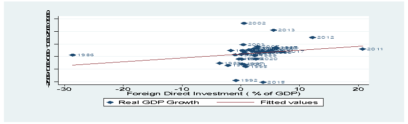
Developing countries are constrained by their domestic investment necessary for sustainable growth of their economies. This is because national savings is not sufficient to support the required investment. This is one of the gaps in the Two-Gap model. This makes the use of foreign capital very important, which can be in the form of indirect investment and direct investment. Foreign direct investment is a sure way to go if the objective is to reduce indebtedness and the risk of sudden capital withdrawal in the form of portfolio investment. The literature on the effect of foreign direct investment on economic growth is huge. Theoretically, creating access to technology or increasing the availability of technology is the core channel of the transmission from foreign direct investment to growth, though it has been noted that the benefit depends on the absorptive capacity of the recipient country, as in Ang (2008). Figure 1.1 shows a scatter plot of Real GDP growth and Foreign Direct Investment (% of GDP) for Sierra Leone. It shows that there is a positive relationship between FDI and growth in Sierra Leone,

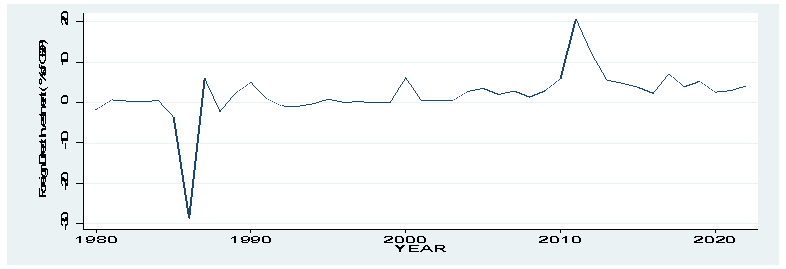
suggesting that more FDI is useful for higher economic growth in Sierra Leone. Figure 1.2 shows that forewing direct investment in Sierra Leone follows a stochastic trend, with increase and decease in foreign direct investments in various years. Hence, while in linear form there tends to be a positive effect of FDI, it is unclear whether periods of increase in FDI and periods of decrease in FDI in Sierra Leone had equal impact on growth, and whether these effects lasted with equal horizons. This is worthy to investigate as it can guide policy makers in terms of balancing the impact of existing FDI firms with attracting more FDI firms. This is useful for local content policy implementation by the Sierra Leone Local Content Agency (SLLCA) and dealing with tax issues by the National Revenue Authority ( NRA) and other policy issues, especially in the mining sector as FDI firms dominates the mining sector, which provides Sierra Leone’s foreign exchange to a large extent.

The paper therefore investigates the effect of an increase in FDI and a decrease in FDI on economic growth in Sierra Leone, to determine whether the effect of FDI on economic growth in Sierra Leone is asymmetric. The result can really reveal where Sierra Leone may lay more emphasis, whether on attracting more FDI, maintaining existing ones or putting equal efforts.

Figure 1.1: Scatter plot of Foreign Direct Investment and Growth in Sierra Leone

Source: World Development Indicators

Figure 1.2: Line Plot of Foreign Direct Investment in Sierra Leone

Source: World Development Indicators

There is a plethora of work on the impact of FDI on economic growth in both developed and developing countries, with a bias for developing countries. In addition, among the studies for Sub-Sahara Africa, focus on whether the impact of FDI is asymmetric or symmetric is not common and such a few studies include Mohamed and Abdulle (2023) for Somalia. However, we are not aware of a published work on Sierra Leone while Kougbaka and Korsu (2025) focused on the linear relationship in Sierra Leone. The importance of the distinction of the effect of an increase and a decrease (asymmetric effect) in FDI on growth lies in the fact that it can establish which of the effects lasts longer and is higher in magnitude. This can guide policy makers in making reforms for sectors with large presence of multinational cooperation, as policy reforms could bring more FDI inflows or make FDI inflow not attractive, which could have implications for existing FDI firms. For example, in some African countries, the extractive industry is the sector that provides the largest foreign exchange and it is dominated by FDI firms, given the huge capital necessary to invest in the sector on a large scale basis. This direction of study is also import because as Sierra Leone implements the local content policies, there is need to know how FDI withdrawal impacts growth of the economy, in other to manage the balance of FDI inflows and national policy reforms that could not be wholly appreciated by FDI operators while they would work towards compliance, which could drag FDI and growth over time.

We organise the rest of the paper as follows: section 2 is the literature review, section 3 is the methodology, section 4 is the empirical results and analysis and section 5 is the conclusion.

2. Literature Review

The literature on the effect of foreign direct investment on growth is huge. This is the case for both sub-Saharan Africa and beyond. The focus has been more on symmetric studies, including Kougbaka and Korsu (2025) for Sierra Leone, Nguyen, (2017)  for Vietman, Younsi, et al (2021), for a group of African countries, and  Salim et al, (2015) for Malasia. However, recently other studies have been considering the asymmetric effect by considering the idea that a negative shock to foreign direct investment may be more destructive than a positive foreign direct investment shock can be constructive. This include the work of Abdi et al ( 2024) for Somalia, Evans et. al ( 2017) for Ghana and Obiokor et al. (2022) for Nigeria.

As indicated in Kougbaka and Korsu (2025), recent studies make use of time series techniques that account for non-stationarity of the variables of a specified growth model while panel dat skills have also been employed.  For example, the study by Nguyen, (2017) in Vietnam from 1990 to 2014 falls in this category, which reveals that FDI inflow has a positive effect on economic growth. Also, Younsi, et al (2021), used panel data techniques for African countries from 1990 to 2016 and the results reveal that foreign direct investment has positive effect on economic growth. The result of Younsi, et al (2021) is similar to Chaitanya, (2009) who used the model specification regression analysis for the period 1980 to 2006 found a positive effect of FDI on economic growth in Latin America, though with small coefficient. The result of Chaitanya (2009) is similar to that of Pandya et al. (2017) in Australia with data from 1980 to 2019 in the sense that the coefficient of FDI is small in spite of a positive effect.

As in Chaitanya, (2009), Nguyen, (2017) and Younsi, et al (2021), Salim et al, (2015) also found a positive effect of FDI on economic growth with data from Malaysia from 2000 to 2010, using the cointegration technique in the context of the ARDL as was the case of Karthikeyan, (2015) who used .Granger causality test, Johansen co-integration test and vector auto-regression (VAR) for India from 2000-2014.

The study conducted by Chisagiu, (2015) supporting the views of other studies from 1992-2012. Multi-dimensional impact of foreign direct investments on the host-economy, determinants and effects, and their contribution to economic growth in Romania and using the Coefficient of Regression Analysis concluded that FDI is one of the strong determinants of Economic Growth rate with significant statistical influence in Romania with high contribution to GDP.

Atrayee et al. (2006) used data from 1993-1998 to investigate the effect of foreign direct investment on economic growth using time series techniques and the result shows that FDI has a positive effect on economic growth. The result of Atrayee et al. (2006) on USA  is similar to  that of Sumei et al, (2008) for China which used data from 1988 to 2003 using  multivariate VAR system with error correction model (ECM), though the latter also revealed that there is only a single-directional causality from FDI to domestic investment and to economic growth in China. The work of Koojaroenprasit, (2012) using data from1980 to 2009 for South Korea, also on a multiple regression basis found that there is a strong and positive impact of FDI on South Korean economic growth. However, Athukorala (2003) with data from 1959 to 2002 for Sri Lanka using the co-integration and error correction regression mechanism found that the regression does not provide much support for a robust link between FDI and growth in Sri Lanka, indicating that FDI investment climate has not improved due to poor governance, political instability, bureaucratic inertia, and poor law and order in the country.

Tatyana (2021) for the G7 countries investigated the role of FDI from G7 countries to  construction and  in Denmark, Italy, Germany, Romania, China, India and Russia from 2005 to 2020 using the Autoregressive distributed lag (ARDL), with co-integration and heteroscedasticity, found that investment in construction supports  growth in the long term.  Another study conducted on the G7 countries by Nawaz Et al. (2024) on from 1990 to 2021 using the annual time series data, autoregressive distributed lags bounds test of co-integration, revealed the existence of long-run relationships among the variables of the model and FDI significantly drives GDP growth, which is consistent with Tatyana, (2021).

Younsi, et al (2021) investigate the FDI-growth effect in African countries with nonlinearities and complementarities from 1990 to 2016 using fixed-effects (FE) and system-GMM estimators, and fond that FDI has a positive effect on economic growth,  as in Agyei et al. (2022) for  Sub Saharan Africa with the non-linear threshold regression analysis.  The result is similar to Adams (2009) on Sub-Saharan Africa from 1990 to 2003, and Njoupougni, (2010), for 36 Sub-Saharan African countries with Pooled Mean Growth estimation from 1980 to 2009, which showed that a one percent increase in FDI induces 0.13 percentage point increase in economic growth.

The study by Ayanwale, (2007), during the period 1970 to 2002, using the ordinary least square investigated FDI and economic growth relationship for Nigeria and found  that the effort of FDI on economic growth may not be significant as the component of FDI do not have a positive impact, but FDI in commercial sector has the highest potential to grow the economy, unlike the study by Zekarias, (2016), which investigated the impact of FDI on economic growth in Eastern Africa from 1980 to 2011, using the dynamic GMM estimators for Eastern Africa  which found a positive effect.

For the asymmetric studies, Abdi et al. (2024) found by applying the non-linear autoregressive distributed lag model introduced by Shin et. al. (2014) with data for Somalia from 1990 to 2020 found that reduce FDI has stronger impact than increasing FDI by the same amount and reduced FDI inflow retards growth while an increase in FDI  increases growth. The result of Abdi et al. (2024) is similar to those of Amin and Liu (2022) for Romania, though the work their work is focused on outward FDI. In Sierra Leone, we are not aware of a study on the asymmetric effect of FDI on growth, while in our earlier paper, the focus was on a symmetric effects.

3. Methodology

3.1 The Model

a) Model Specification

The model estimated draws from the endogenous growth model Romer (1990), Grossman and Helpman (1991) and Barro and Sala-i-Martin (1994)), which has been adopted and modified by other studies to suit economy structures, including  Borensztein (1995).  Moreover, Mencinger (2003), Lee and Tcha, (2004), Carkovic and Levine, (2002) have indicated that foreign direct investment is conducive to growth because it creates the opportunity for more investment in infrastructure for growth.  The opportunity to have access to technology transfer has been given as a channel for the importance of FDI to growth, as in Borensztein et al. (1998) and Lim (2001). Hence, with GROWTH representing growth of real GDP, FDIGDP representing foreign direct investment (% of GDP) and t representing time subscription, equation (3.1), is the simplest form of the model estimated.

GROWTHt=FDIGDPt                                                         (3.1) 

However, as a decline in FDI and an increase in FDI may be associated with different magnitude of effect and length of impact, which implies an asymmetric effect of FDI on growth, we split FDIGDP  to have a variable representing increase in FDI, which is FDIPOSGDP, and one representing decrease in FDI, which is FDINEGGDP. Thus, equation (3.2) reflects the adjustment to equation (3.1).

GROWTHt=FDIPOSGDP, FDINEGGDPt                                      (3.2)

We introduce trade openness in order to capture the role of opening up Sierra Leone to trade on economic growth. Based on the Keynesian aggregate demand, a priori, when imports increase aggregate demand reduces while increase in exports increases aggregate demand for domestic output. The former detracts from output and the latter increases it. The combined effect depends on the relative impact of the import and export effects. However.  Krueger and Berg (2003) and Lopez (2005) have noted that trade openness creates the opportunity to use improved technology and it brings access to larger markets, making firms to capture opportunities out of the home location.

We also introduce terms of trade, as noted by Bleaney and Greenaway (2001), Blattman et al. (2003) and Urban (2007), that terms-of-trade has a positive effect on economic growth due to relative price effect: when a country's export price increases relative to its import price, income increases because exporters have higher income for the same quality of goods. When import price falls, importers can afford more imports without spending more. This improves access to capital goods, technology, and raw materials, thus increasing income by increasing domestic production.

As observed by Stockman (1981), Fischer (1983), Barro (1995) and Valdovinos (2003), higher inflation theoretically serves as a loss to macroeconomic performance by providing an unfavourable background for sustainable growth. Inflation is expected to have a negative effect on economic growth as it discourages savings and erodes real value of assets. Higher inflation may lead to higher uncertainty about economic prospects. This may make investors exercise a wait and see option, as in the Real Option Theory of Investment. This has also been pointed out in   Zilibotti (2001) and Vinayagathasan (2013). Thus, we introduce inflation in the theoretical model

We also introduced the real exchange rate in the model, as real exchange rate depreciation is expected to increase competitiveness of an economy to international trade by increasing export and reducing import. Thus increasing aggregate demand and output. McKinnon (1964) Fletcher (1994), Crompton et al, (2001), and Surugiu (2009) have identified how this channel works. Considering these adjustments to the basic model in equation ( 3.1), equation (3.2)  shows the theoretical model estimated.

GROWTH=FDIPOSGDP, FDINEGGDP, OPN, TOT, REER, INF                                                    (3.2)

Where GROWTH is real GDP growth, OPN is openness of the economy to trade, TOT is terms of trade, REER is real effective exchange rate and INF is inflation rate, FDIPOSGDP is increase in GDP and FDINEGGDP is decrease in GDP.

In light of these considerations, the non-linear (asymmetric) dynamic model is given as in equation (3.3).

GROWTHt= φ+0p1βiFDIPOSGDPt-i+0p2θiFDINEGGDPt-i+0p3πiOPNt-i+0p4τiTOTt-i+

 0p5σiREERt-i+0p6μiINFt-i+1qγiGROWTHt-i+Ut        (3.3)  

  Where  FDIPOSGDP    and  FDINEGGDP  are essentially the cumulative partial sum of the positive changes and negative changes in FDI (percentage of GDP), which are obtained as in Shin et. al      (2014).  This is given as follows:

That is,  FDIPOSGDPt=t=0t=iMax  ∆FDIGDPt,0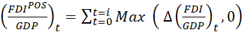                                             (3.4)

Also,      FDINEGGDPt=t=0t=iMin  ∆FDIGDPt,0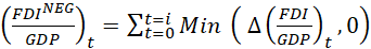                                             (3.5)                                

 With this transformation, the following always holds:

               FDIGDPt=i  = FDIGDPt=0  + FDIPOSGDPt=i  +FDINEGGDPt=i                        (3.6)    

3.2 Estimation Technique

In the estimation of the model, consideration was given to the fact that estimation in dynamic form is preferred to a static model estimation as it provides opportunity to measure persistence of real GDP growth, it captures delayed effects of regressors. It also ensures that autocorrelation is not swept under the rug by basically adjusting standard errors since lag length misspecification errors can be a major source of autocorrelation. Hence, a dynamic model was estimated with initial lag length of three for each variable. The choice of maximum lag was meant to gain on degree of freedom.

In the estimation, all variables that were not stationary were transformed to achieve stationarity status in order to avoid spurious correlation, this was done for terms of trade, which was stationary only after first difference while the rest were found to be stationary. The augmented Dickey Fuller Generalized Least Squires (ADF-DLS), which detrends the original series and applies the orginal Augmented Dickey-Fuller (ADF) test to it was applied. However, a varaible that has structured break may reveal not stationary with the ADF-GLS test, when in-fact it was stationary. Thus, it leads to high probability of failing to reset the null hypothesis of the existing unit root against the alternate of no unit root (stationary). Thus, we employed the Perron-vogelsang test (a single break test) and the clement Montare-Reyes test (a double break test).

A parsimonious model was searched for based on the Hendry’s general to specific modelling framework and it was tested for series of model diagnostics that are to be done when the ordinary least squires is applied to stationary series. There are residual normality, autocorrelation, heteroscedasticity and parameter stability test.

3.3 Data Sources and Description and

Table 3.1 shows the description of model variables and sources of the data.

Table 3.1: Data Sources and Description

4. Empirical Results
   1. Descriptive Statistics of Model Variables

Table 4.1 shows the descriptive statistics of all model variables, which reveals that the mean growth of real GDP is 2.68 with a medium of 3.75%, implying that there were very low growth figures during 1980 to 2024 that drove the mean growth to be below the median. Essentially, most of the growth figures of Sierra Leone are above the mean growth of 2.68%. For FDI (% of GDP) the distribution follows that of real GDP growth, having a heavy tail to the right of the median, as the mean is 1.94% of GDP, which is below the median of 2.02% of GDP.  For increase in FDI, the mean is 52.51 and median is 52.57, Hence, the are almost equal number of observations to the right and left of the mean as in the case of the median, unlike decline in FDI, which has more observations to the right  the mean of 48.29 % of GDP, as the median is 50.4 % of GDP % of GDP.

In the case of trade openness, terms of trade and real effective exchange rate and inflation, their mean values are higher than their median values. This implies that there are large values to the right of the median (higher than the median), that drive the mean to the right of the median leading to higher mean values. In terms of the variability of these variables, as measured by the coefficient of variations, FDI (% of GDP) is the most volatile variable, followed by real GDP growth and inflation rate with coefficient of variation of 3.15%, 2.98% and 1.15% respectively, while trade openness is the least volatile one with coefficient of variability of 41%, followed terms of trade with 53% and real effective exchange rate with 68%.                     

Table 4.1: Descriptive Statistics of Model Variables

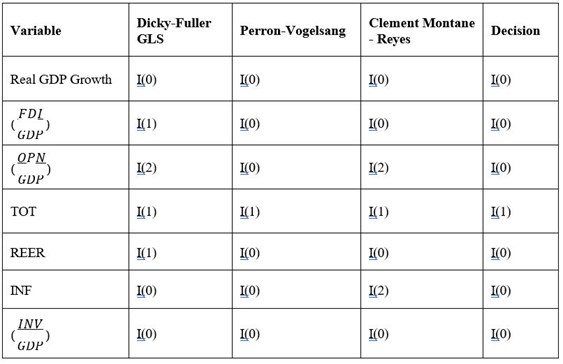
We investigated the stationarity of each model variable in order to avoid spurious regression in the application of the Ordinary Least Squares (OLS). A battery of stationarity (unit root) tests were applied. Specifically, the modified version of the Dickey-Fuller test, (Dickey Fuller GLS) was applied. This was supplemented with structural break tests that account for one and two breaks, which are the Perron-Vogelsang test and the Clement-Montanes-Reyes test. Appendix Tables 1, 2 , 3 show the unit root test results of the various tests and Table 4.2 show the summary results of the test. It shows that all but one variable is stationary in level. The exceptional variable is Terms of Trade, which is stationary after first differencing.

The decision criteria out of the many tests is that when a variable has a lower order of integration based on a non-structural break test, then it is integrated with that order. Otherwise, the order of integration dictated by a structural break unit root test is considered, and a test with two structural breaks is more robust than one with only one break, except if the one break test has a lower order of integration. This is because structural break may render a variable to appear non-stationary by the Dicky Fuller- GLS test while one break may also it to appear non-stationary if there are two breaks.  

4.3 The Estimated Model Results  

The Ordinary Least Squares is employed with terms of trade entering in its first difference form and all variables entering the model initially with two lags as maximum lag. Table 4.3 shows the estimated model results in parsimonious form, which is the result with insignificant variables eliminated. Two forms of the model were obtained, first, the model where all FDI terms are included in spite of their insignificant levels, which is model 1, and then the form where all insignificant variables, including the FDI terms, are eliminated, which is given by model 2.

The estimations with the exclusions of all insignificant variables (Model 2), including the FDI terms, has lower Akaike-Information- Criterion (AIC) and lower Bayesian Information Criterion (BIC), which are 261.27 and 276.47, respectively, compared to AIC of 263.97 and BIC of 284.24 respectively for the alternative model (Model 1 ). Also, the adjusted R2 for Model 2 is 0.5378, compared to 0.5286 for Model 1. We therefore select Model 2 as our congruent preferred parsimonious model of growth with asymmetric effect of FDI

Table 4.3: The Economic Growth Model with Asymmetric FDI Effects

*** p<0.01, ** p<0.05, * p<0.1

The estimation model result (Model 2) shows that there is no persistence in economic growth in Sierra Leone. This is because the lag coefficient of growth is not significant and is negative. The model results also reveal that when FDI increases in a year, after one year its impact on economic growth in Sierra Leone is positive, with impact coefficient of 0.72 and is significant at the 1% level. The model result also shows that, when FDI decreases in a year, in the following year, economic growth increases, since the sign of the one year lag coefficient of FDI is negative with impact coefficient of -0.94. However, after the second year, economic growth declines with an impact coefficient of 1.58. The sum of these two coefficients (-0.94+1.58) is 0.64. H. It is thus observed that when FDI increases in Sierra Leone, its increasing-growth effect is felt after a year and when it decreases its decreasing growth effect is felt after two years and is more than doubled (a coefficient of 1.58) the positive one-year impact of an increase in FDI (a coefficient of 0.72).

Also, for every one-percentage point decline in FDI in a given year, there is a 0.64 percentage point decline in growth of real gross domestic product from the 1^st to 2^nd year.  Therefore, in Sierra Leone, the impact of FDI on economic growth is asymmetric with the first year impact of an increase in FDI being growth enhancing, the first year impact of reducing FDI being growth enhancing. However, in the second year, the impact of reducing FDI is substantial and disastrous since it is more than the initial positive effect of the increase in the FDI and the growth model declining effects comes much later in the second year of the decline in FDI.

4.1 Model Diagnostic Tests

Model 2, which is the preferred model was subjected to various diagnostic tests to ensure model validity (Column one of Table 4.4). As the Ordinary Least Squares is applied with transformation of the non-stationary variable, tests for normality of model residuals, serial correlation, heteroscedasticity and parameter stability test were employed. Table 4.4 shows the model diagnostic tests, which shows that the model is free from serial correlation, heteroscedasticity and poor functional form. Also, as shown in Figure 4.1, the model parameters are stable.

Table 4.4: Diagnostic Test of Model Residuals for the three Models

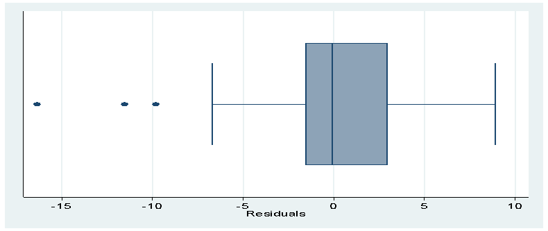
However, the diagnostic test results shows that the model residuals are not normal, requiring further motivation. The box plot of the model residuals is shown in Figure 4.2, which shows that there are cases of extremely low values of real GDP growth as there are observations below the lower whisker of the box plot.

Figure 4.2: Box Plot of Model Residuals

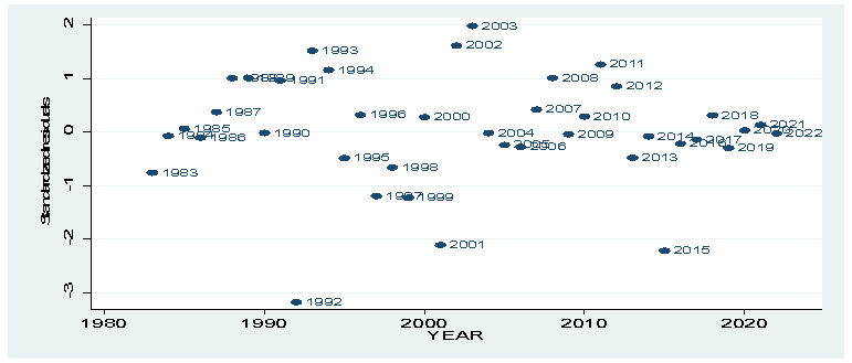
Figure 4.3 shows a scatter plot of the standardized residuals, which shows that in the years 1992, 2001 and 2015, the standardized residuals are lower than two standard deviation of the mean, implying that the growth rates in these years were lower than dictated by the model fundamentals. The year 1992 was a year old, following the start of the rebel war in Sierra Leone (1991 to 2001). In 1992, the destruction of capital and labor had been extended with shrinking of agriculture, the then main contributor to real GDP and investor confidence had eroded, as the main diamond mining District fell under rebel control. At the time. Diamond was Sierra Leone’s main export and a large part of the rural areas of Eastern Districts of Kailahun and Kenema and the Southern District of Pujehun had had shrunk agricultural production, with the attendant expectation of growth prospects revised downwards by major actors and analysts. The year 2001 was still a war period though it was about the end of the war and 2015 was the Ebola Virus Disease year, which started in the second quarter of the year. It was a year of loss of many lives and the lockdowns to gain on the health battle provided economic loss to the nation, culminating into welfare loss and direct loss of the overall output of the economy. Thus, real GDP growth rates in 1992, 2001 and 2015 were -19.01%, -6.35% and -20.49%, respectively, which were below the mean and median of 2.68% and 3.75%, respectively, during the period 1980 to 2024 and the mean and median of 2.57 % and 3.47 % respectively, during 1980 to 2022. The associated standardized residuals are -3.17, -2.11 and -2.21 for 1992, 2001 and 2015, respectively.

Figure 4.3: Scatter plot of the standardized residuals