1.Introduction:

Agriculture in developing countries is influenced by a wide range of climate, ecological and topographical diversities, is the backbone of the economy of these countries with more than 60% of the working population engaged in this sector. The dependence of the majority of the farmers on rainfed agriculture and pastures has made the economy extremely vulnerable to the vagaries of the weather and climate. As a result, failure of rains and the occurrence of drought during any particular growing season lead to severe food shortages. Thus, in developing countries early warning of food crop situation and impending drought situation is very important to make timely decisions on relief and rehabilitation to affected population and to take several other appropriate decisions by different government and non-government Agencies. In the case of developing countries, most of the production comes from family sector. In addition to this, the other major crop production sector is state farms. There are several other sectors like cooperatives, but they can be grouped under one of these two major sectors, based on the existing practices in a given country.

Family sector agriculture represents the conventional [traditional] farming system of agriculture mainly with low inputs & poor management on small holdings [with irregular terrain] while the state farms agriculture represents the improved system with high inputs & better management on larger regular terrain. The latter is more influenced by the latest changes in agricultural system. Thus, the early warning procedures should be separated for these two sectors. The author formulated a procedure for family sector agriculture with reference to Mozambique (Reddy, 1989) for the early warning of crop yields and drought monitoring using water balance model. The model was tested for Ethiopia in Africa (Reddy, 1991). Some basics on drought were presented in Part – I (Reddy, 2022).

2.Methodology: Materials & Methods:

2.1. Introduction:

One must clear the fact that the research results do not fit in to reality in farmers’ farms. The research results must help to understand the weather relation to yield. Past such results clearly showed they are not linear, but they follow the curvilinear pattern. The temperature, radiation & moisture presents linear or nearly linear in an optimum range and at the two extremes present more or less flat like steps in a house [flat, rising and flat, Reddy, 1995]. However, the optimum range varies with crops (Reddy, 1993), soils and relative humidity conditions. To overcome these limitations under field conditions Reddy (1989) proposed a concept with reference to Mozambique for crop early warning system for yield and drought monitoring and later adapted to Ethiopia (Reddy, 1991).  

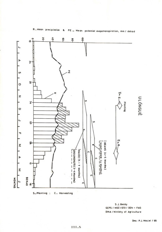
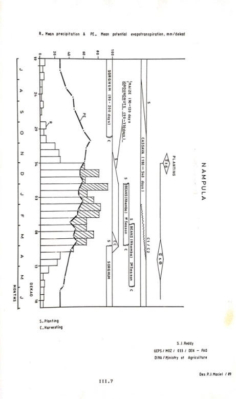
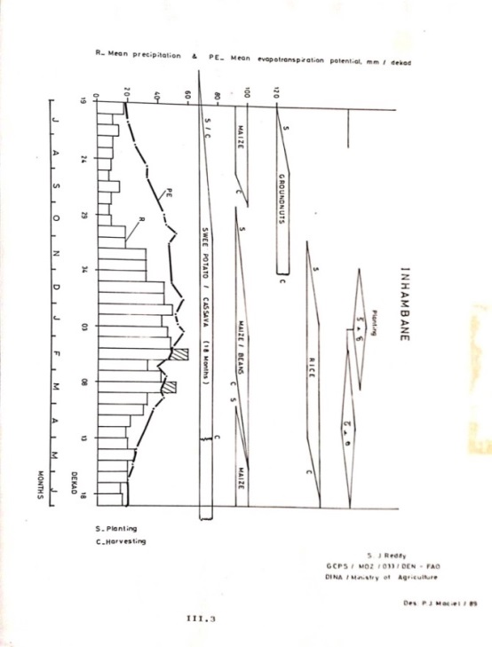
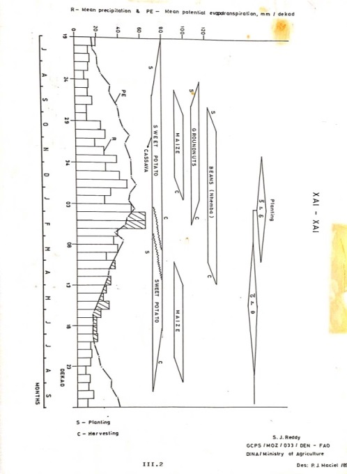
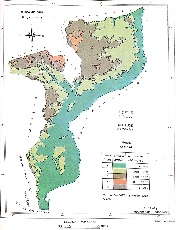
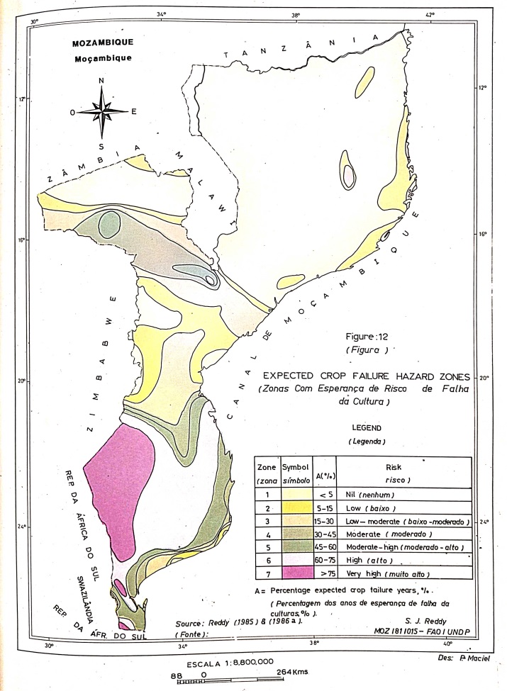
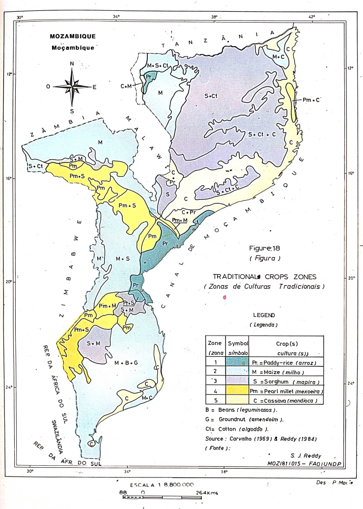
After carrying out the base work and other information at district level on family size, area per family, & percentage area occupied by crops along with the crop calendar. Reddy (1984, 1986a, 1989) presented all the basic information on soils, crops, etc. Annexure-I presents the rainfall, potential evapotranspiration, crops calendar for 7 regions [Lichinga, Ulongue, Tete, Nampula, Quilimane, Inhambane & IAX-IAX] in Mozambique representing from north to south. Horizontal scale represents from decade 3 to decade 3. The rainfall and potential evapotranspiration showed wide variations and accordingly the crops grown in those provinces. However, African countries showed natural rhythmic variations in rainfall (Reddy, 1993). By linking projected future expected patterns, prediction of yields and drought conditions will improve the results of the model. Reddy (1986b) & Reddy & Mersha (1990) presented natural variability in rainfall of Mozambique and Ethiopia, respectively. Here soil also play important role in the selection of crops – for example in sandy soils root crops and maize in Vertisols. Annexure-II presents 8 Maps presenting basic data such as terrain, soils, climate and crops in Mozambique. The procedure for the early warning of crop yields/production and drought monitoring has three major components, namely:

1. Identification of model for the estimation of weather index
2. Development of model that relates weather index to yields of individual crops
3. Development of procedures for crop early warning and drought monitoring

These are discussed below.

2.2. Development of model that relates weather index with grain yields:

2.2.1. Introduction:

For the estimation of model that links the weather index or water stress index that relates to crop yields, it is essential to have a suitable water balance model. ICSWAB model’s (Reddy, 1983a) predictive ability of stress under rainfed dry-land condition was found to be good (Reddy, 1983b). However, this is o.k. as far as state farms are concerned but under family sector, where large variations are seen in rainfall, crop varieties - planting/cropping system, management practices, soil types/slope, etc. such a sophisticated model may not be the right choice. Under this condition models such as FAO water balance model (Frere & Popov, 1979) is more appropriate.

2.2.2. Procedure for the estimation of weather index:

Symbols:

I                       =          Water requirements satisfaction index, %

[Weather index or water stress index varies between 100 and 0 with 100 at planting dekad – month is divided in to three10-day/dekad intervals]

AWC               =          Water holding capacity of the soil in the top 1.8m depth of the soil, mm

Kc                   =          Crop coefficients

R                     =          Rainfall [Ry = current; Rn = normal], mm

PE                   =          Potential evapotranspiration [PEy = current; PEn = normal], mm

RPB                =          Minimum rainfall amount expected at 75% probability level, mm

                                    [Estimated using incomplete gamma model]

SM                  =          Soil moisture reserve, mm

D                     =          Water deficit, mm

S                      =          Water surplus, mm

WR                  =          Water requirement, mm

TWR               =          Total [planting to harvest] water requirement, mm

FWR               =          Future water requirement, mm

FWA               =          Future water availability, mm

AE                   =          Actual evapotranspiration, mm

E                      =          Open pan Class “A” evaporation [with mesh cover] –

Ey = current & En = normal --, mm

AE/E               =          Relative evapotranspiration

SM/AWC        =          Relative soil moisture reserve

RO+D             =          Runoff [surface runoff + deep drainage], mm

Y                     =          Actual yield, t/ha

Yo                   =          Potential or maximum yield, t/ha

Ya                   =          Average yields [Yo = 2 x Ya], t/ha

I                       =          Current period (day or dekad]

TDM               =          Total dry matter production, kg/ha

F                      =          Superphosphate level, kg/ha

Input data:

Weather factors at dekad/10-day interval – a month is divided in to three dekads -- [R (Ry & Rn) & PE (PEn) & RPB]; soil factor [AWC]; crop factor [crop type, crop growth cycle in dekads (planting to harvest), planting dekad & crop coefficient];

R: rainfall is recorded at a good number of stations and thus it represents the observed data [both current dekad (Ry) and normal dekad (Rn) estimated based on historical data];

PE: Potential evapotranspiration needs to be estimated from other meteorological parameters. For example:

1. If open pan Class “A” evaporation data are available, then PE = 0.85 x E (with mesh cover) or PE = 0.75 x E (without mesh cover)
2. Using Penman (1948) model as outlined by Frere & Popov (1979) estimate PEn from normal climatic data such as daily average temperature, relative humidity, wind speed and hours of bright sunshine. Under this if sunshine data are not available then this parameter can be estimated from the daily average total cloud amount using the procedure of Reddy (1974).
3. Estimate PE using (i) and/or (ii) wherever the necessary input data are available and then using these PE estimates, develop regression equations of the form (Reddy & Neto, 1984; Reddy, 1991):
   1. Pen = a + b x la +c x lo + d x h + e x Rn’, where a is the regression constant, b, c. d & e are regression coefficients for la = latitude in degrees, lo = longitude in degrees and Rn’ = [Rn + Rn”/3]^1/3 in which Rn is the normal rainfall of the month and Rn” is the normal rainfall of the previous month
4. Procedure (iii) can also be used for the estimation of individual years PE values (PEy) by using Ry in place of Rn or alternatively from PEn, estimated from procedure i to iii, PEy values can be inferred following the procedure of Reddy (1979) as:

[PE]_I = [PEn]_I x [1.0 ± 0.06 x |Z_i|^1/3 where |Z_i| is the absolute value of Z_i = 0.7 x {[Ry – Rn]_I + [Ry – Rn]_i-₁/3}; if Z_i > 0 then -0.06 or if Z_i < 0 then 0.06

Crop coefficient [Kc]:

FAO (1986) & Frere & Popov (1979) presented few examples of Kc for different crops. Figure 1 presents the schematic presentation of crop coefficients (Kc) with reference to growth stages of a crop. Reddy (1983a) presented crop coefficients for sole crop, intercrop and double crops under ICSWAB model (Reddy, 1983b). Table 1 presents the values of crop coefficients (Kc) at different growth stages for few selected crops as an example. For individual dekads, Kc values have to be interpolated, as explained in Figure 1. Crop coefficients can be adjusted to local crops/varieties by deriving growth stage durations [f1 to f5] from method presented by Reddy et al. (1984).

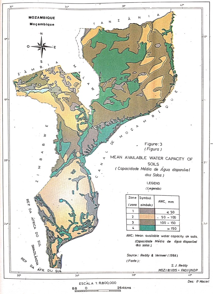
AWC: AWC = [FC – WP]_{0 – 0.9} + {[FC – WP/2}_{0.9 – 1.8}, where FC is the field capacity and WP is the wilting point, respectively given by -0.3 and -15 bars. The water retained in mm between field capacity and wilting point in the top 90 cm of the soil plus the 50% of this in the 90 to 180 cm depth of the soil [if the soil exists upto that depth]. Reddy & Vermeer (1984) estimated available water capacity of the soils of Mozambique. The map depicting these estimates is presented in Annexure-II.

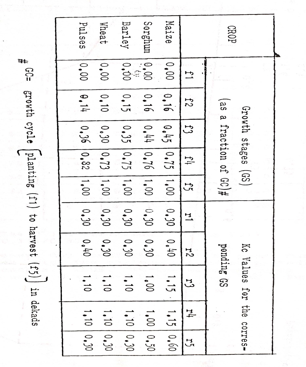
Table 1: Kc values vs growth stages for few crops in Ethiopia

 

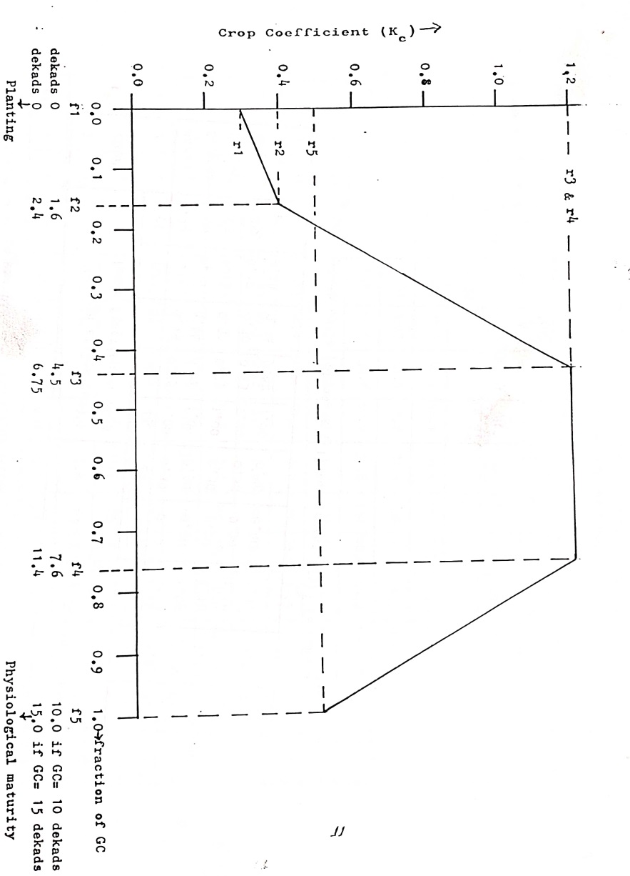
Figure 1: Schematic presentation of crop coefficients (Kc) with reference to growth stages of a crop

Procedure for the estimating weather index:

Step 1: Compute the total water requirement [TWR] as:

TWR   =          j=1iPEy x Kc_{j    +  j=1+1kPEn x Kcj}                                               (1)

Where j = i refers to planting dekad and j = k refers to the harvesting dekad.

Step 2: Compute water requirements [WR] for a given dekad I as:

WR_i     =          [PEy x Kc] _I                                                                                                      (2)

Step3: Compute rainfall deficit or surplus (WR’) for a given dekad i as:

If WR’I > 0 then surplus or if WR’_I < 0 then deficit; The surplus goes to the soil moisture reserve and/or runoff or if deficit, then equivalent to this amount is extracted from the soil moisture reserve and/or plant suffers due to deficit water supply.

Step 4: Compute the soil moisture change (SM) for a given dekad i as:

SM’_I    =          SM_i-1 + SM’_i                                                                           (4)

If SM’_i < 0 then D_i = SM’_i ; SM_i = 0 & S_I = 0                      

If SM’_i > 0 then S_i = SM’_i  - AWC; SM_I = AWC & D_I = 0

If 0 ≤ SM’_I ≤ AWC then S_i = D_i = 0 & SM_i = SM’_i 

Step 5: Compute water requirements satisfaction index (I) for a given dekad I as: 

(i)         on planting dekad I₁ = 100%

(ii)        if deficit then I_i = I_i-1 - [D_i/TWR] x 100

(iii)       if surplus than I_i = I_i-1 – 3 x P

            Where P = 0 if S_i < 100 mm

                        P = 1 if 100 ≤ S_i < 200 mm

                        P = 2 if 200 ≤ S_i < 300 mm, etc.

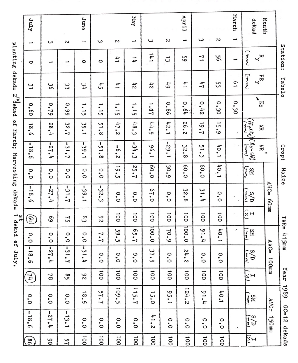
Table 2: Water requirement satisfaction Index (I) under three soil water holding capacities in Ethiopia [Yabelo]

Step 6: Compute the future water requirement [FWR] & future water availability [FWA] for dekad i+1 as:

FRW_i+1 = [PEn x Kc]_i+1          and  FWA_i+1 = SM_i  + RPB_i+1

In this model, I represent the weather index or water stress index. It varies between 100% (no stress) to 0% (no crop).

In 5(ii) above, deficit (D_i) = [PEy x Kc] _I – AE_i, where Kc acts as a non-linear adjustment to PEy at each dekad and thus water stress term is termed as non-linear additive multiple stage model. Table 2 presents an example of computing water requirements satisfaction index (I) under 3 soil types [AWC = 60, 100 & 150 mm]. It is seen from the table that I for AWC = 60, 100 & 250 mm respectively are 64, 74 & 86 [Reddy, 1991].

1. 1. 3. Discussion – FAO model vs ICSWAB model:

ICSWAB model uses daily data while FAO model uses 10-day or dekad data. In the case of FAO model, the water use is estimated relative to PE while in ICSWAB model they are estimated relative to E, where PE = 0.85 x E. Both the models use water holding capacity of the soil (AWC or K), however in the case of FAO model this acts as a storage while in ICSWAB model it is used as storage as well as water extraction rate depends upon this factor. Both the models use crop coefficients but in difference sense. For example:

In the case of ICSWAB model crop coefficients (b_i) are developed based on leaf area index and % light interception to reflect the root growth and thereby it accounts the water extraction rate at different growth stages. But here crop coefficients do not limit the water use. That is, under rainfed condition if more or less every day rains occur, and this rain is more than or equal to the evaporative demand then the water extraction is at potential rate irrespective of crop coefficient or soil type. This is not the case with FAO model.

In the case of FAO model crop coefficients (Kc) are related to the maximum amount of water expected to be extracted by a dry-land crop during post-rainy season [without rains or irrigation] with sufficient reserve in the soil (PC) to that of evaporative demand (PE). This is given as: [Kc]_I = [PC/PE] _i

Here, the water use is restricted by Kc. But this factor indirectly accounts the growth stage effect on water stress as related to yield (Reddy, 1983b). In ICSWAB model, this has to be accounted through the yield function. In FAO model, the growth cycle [if it is a dekad] is divided into n-1 growth stages while in ICSWAB model this can be divided as many stages as possible, as it is given at daily interval.

The differential water extraction patterns (PE in place of E and Kc x PE in place of E), limits the use of FAO model under state farms as it overestimates the water use at latter growth stages by storing more water, particularly under dry climates. However, this may not be significant for crops grown on conserved soil moisture [Reddy, 1983a] in post-rainy season and also under family sector may not be a limitation when compared to the local variations as outlined earlier.

The Kc values, in FAO model to account the water extraction, given in Table 1 are too generalized values but they need to be adjusted for seasons in which plantings are undertaken or growth is completed and for plant density. These variations are directly accounted in ICSWAB model [Reddy, 1983b]. Therefore, it is suggested to adjust the Kc values under rainfed agriculture as:

Case i: Planting at the start of rains and harvesting at the end of rains: It assumes that if water is available most of the dry-land crops extract water at the same rate. Under this condition soil evaporation is present.

f           1          2          3          4          5          Plant density

r           0.30     0.40     1.20     1.20     0.50     high

            0.30     0.40     1.10     1.10     0.40     moderate

            0.30     0.40     1.00     1.00     0.30     low

Case ii: Planting in the middle of the rainy season and harvesting in post-rainy season [i.e., last phase of f4 – f5 is in dry season]]. Soil evaporation is negligible during the last phase (f4 – f5).

f           1          2          3          4          5          Plant density

r           0.60                 1.20     1.20     0.00     high

            0.60                 1.10     1.10     0.00     moderate

            0.60                 1.00     1.00     0.00     low

Case iii: Planting at the end of rainy season and harvesting in the post-rainy/dry season [crops grown on conserved soil moisture only]. Soil evaporation is negligible.

f           1          2          3          4          5          Plant density

r           0.30                 1.00     1.00     0.00     high

            0.30                 0.90     0.90     0.00     moderate

            0.30                 0.80     0.80     0.00     low

Similarly based on local conditions/crop varieties define f2, f3 & f4, particularly f4 & f5 – start and end of flowering/reproductive phase.

Reddy et al. (1984) presented a method to estimate the durations of three phrenological phases for a crop/variety. Based on such estimates Kc values can be derived for specific cases.

1. 1. 4. Crop yields vs weather index functions:

Under family sector: (a) grain yields refer to a region (for example a district) while the weather index refers to a location or group of locations in that region. The relationships between yield and weather index for few cases were presented by Frere & Popov (1979) and FAO (1986) using FAO water balance model. Reddy (1989) presented functions in the case of Mozambique; (b) data set: for developing such functions one needs either historical data or for few years from a well distributed network of stations with reference to crop and climate and as well as the information on soils. In the case of Mozambique Reddy (1989) used the historical data [1944-‘66] of 8 districts under different agroclimatic/ecological zones – Reddy (1989) book includes maps of soil, climate, crop, etc. parameters; (c) functional form: The relationship between the weather index and yield is expressed by a function. The selection of this functional form is critical for the successful implementation of crop early warning in any given country.

The integrated function of Yc/Ym as a function of Ic, by forcing the curve to pass through the origin [assuming yields are zero where Ic = 0] is given in Figure 2. This curve is expressed as:

[Yc/Ym] = [{10/ (100 – 0.9 x Ic)} + {(Ic/1000) – 0.1}]

Few important issues are estimation of average index (I) at district level under (a) different planting dates of a given crop, (b) different soils [see Table 2], etc. These are explained by Reddy (1993).

Figure 2: Variation of relative maize yields (Y/Yo) with requirement satisfaction Index (I)

Generally, the yields show high specificity with respect to crop variety/ cropping system/management practices/inputs on one hand and with soil type/slope and/or agroclimatic zones/regions/location/altitude, etc. on the other. All these means that even for the same weather index the yields are different under different altitude zones/agroclimatic zones (Reddy, 1989), soil types (Reddy, 1983b); crop variety (Frere & Popov, 1979); cropping system (Reddy & Morgado, 1987); etc. It was observed by Reddy (1989) that this specificity could be minimised by considering relative yields [Y/Yo] in place of yields [Y] while comparing with weather index (I). Then the crop early warning procedure with special reference to family sector was designed. Relative yield [Y/Yo] is expressed as a function of water requirements satisfaction index in % [weather index or water stress index varies between 100 and 0 with 100 at planting decade] (I).  Index of water requirements satisfaction (I) will reflect the cumulative water stress/excess water encountered – estimated through crop-soil water balance model -- by the crop dekad after dekad. The higher the final index the smaller is the water stress/excess water hazard. This index has a relationship with the final yield. Yields could be estimated per crop per district by multiplying the average integrated Y/Yo values obtained by Yo.  In Figure 3 using the historical data, checked the validity of the model Y/Yo vs I before actually using this model in any given country (Reddy, 1989 & 1993).

Figure 3: Variation of maize yields under family sector with water requirements satisfaction Index and agroclimatic classes

Table 3 presents the variation of average yields (Ya) with 5 agroclimatic zones (C) – Each district was characterized by its C value that provides the integrated index of climate – which accounts for the variable soil and climate conditions. This is represented by the following equation.

Ya = 0.9577 – 0.0264 x C²

 The 5 agroclimatic zones are characterized as follows:

Class 1, the risk of crop failure due to drought is < 5%         -- excellent

            Intensity (%) cropping 200% -- double cropping 100% of years

Class 2, the risk of crop failure due to drought is 5-15%- very good

            Intensity of cropping 140% - double 25 & inter 75% of years

Class 3, the risk of crop failure due to drought is 15-45% --good

            Intensity of cropping 100% --inter 100% of years

Class 4, the risk of crop failure due to drought is 45-60% -- moderate

            Intensity of cropping 80% -- inter 75 & single 25% of the years

Class 5, the risk of crop failure due to drought is > 60% -- poor

            Intensity of cropping 60% -- single 100% of years

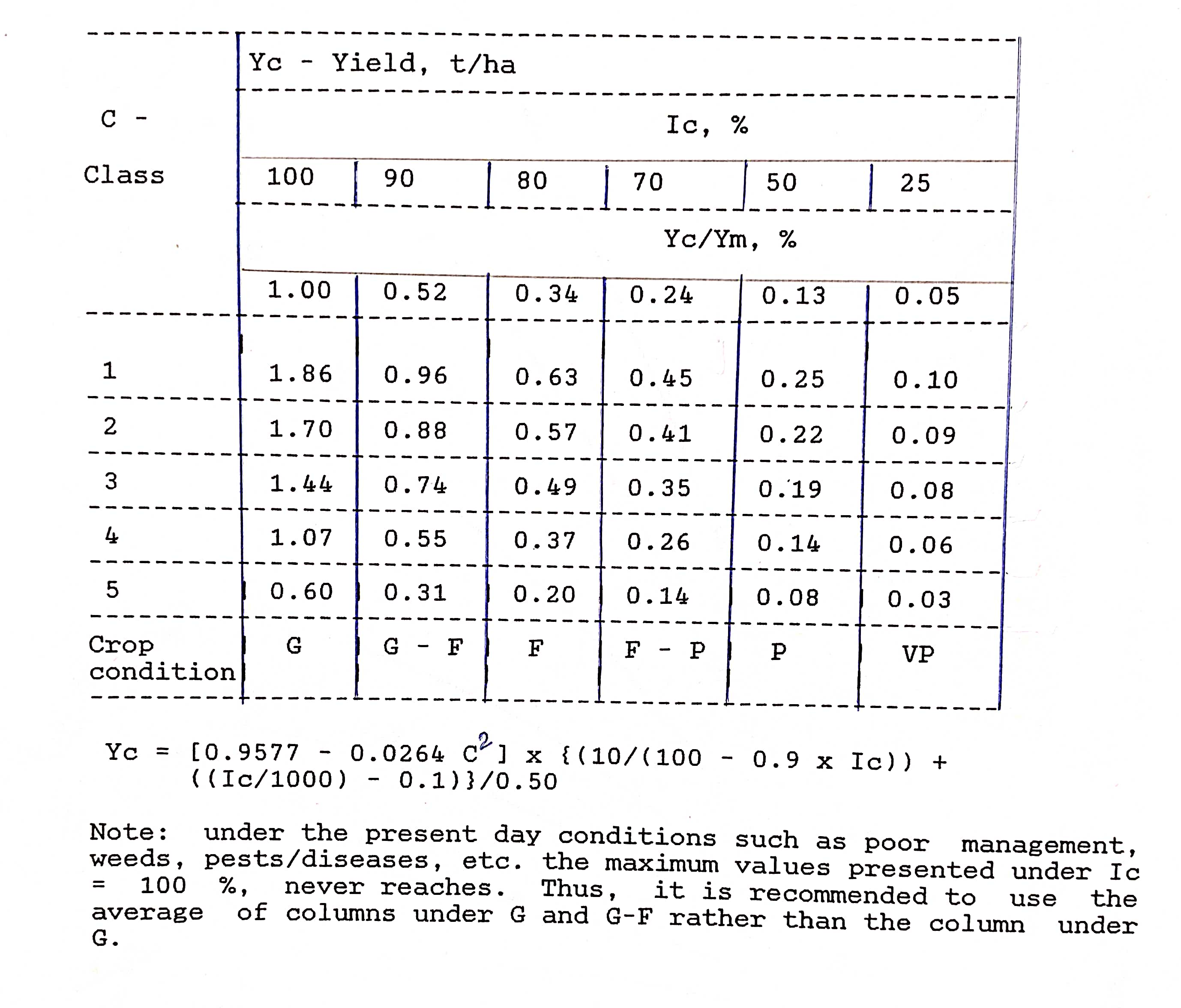
Table 3: Climatically possible yields of maize under family sector [Figure 2]

According to these, the yields are agroclimatic zone dependent. Thus, in order to present the yield levels representative of five agroclimatic zones and Ic, the curve in Figure 2 and Table 3 for C are integrated in terms of maximum yields obtained from the 8 districts data (Ym = 1.86 t/ha). These are presented in Figure 3 under the 6 ranges of Ic presented in top table in Figure 2. Table 3 presented these values.

Ranges are used because in the yield estimation Ic values of a single met station are assumed as representative of a region. In order to nullify the local variations of that region this technique is used. Yc/Ym is used as = 0.5, which other words means average condition. This means, Yc = Ya for agroclimatic zones 1 to 5 for Ic in the range of 90-80%. Then linearly extrapolate for Yc/Ym = 1.0, 0.52, 0.34, 0.24, 0.13 and 0.05 corresponding to the remaining 5 intervals of Ic. The integrated equation for Yc is given as:

Yc = (0.9577 – 0.0264 x C²) [{10/ (100 – 0.9 x Ic)} + {(Ic/1000) – 0.1}]/0.50

Note: under the present-day family sector, the maximum value never reaches due to several reasons such as poor management, weeds, pests/diseases, etc. Thus, it is suggested that use the average Yc values of G and G-F rather than G values of Yc when Ic is 90-100% range.

3. Results: Procedures & Discussion:

The curve in Figure 2 was compared with the data of pearl millet experiments at Niamey/Niger [Figure 4], with the observed data from Ethiopia for wheat and sorghum under different climatic conditions [Figure 5], with the experimental results of two groundnut varieties at Bambey/Senegal and regional sorghum yields from different regions of Botswana of different years [Figure 6] (Reddy, 1993; FAO, 1986). In all these cases, in general, the observed data are very close to the curve in Figure 2.

Figure 4: Comparison of crop yield function of Mozambique with the pearl millet data of Niamy/Niger

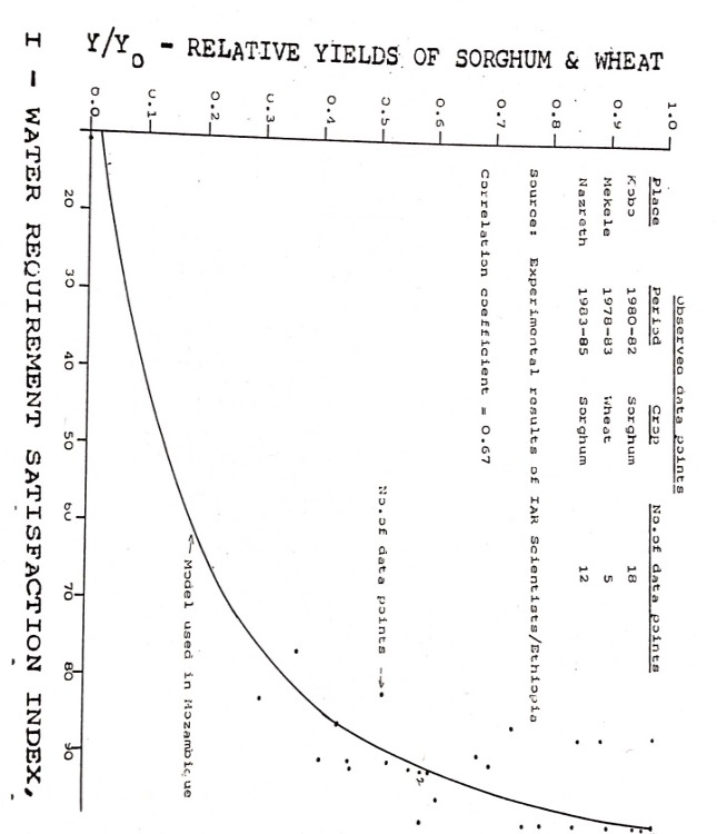
Figure 5: Comparison of crop yield function of Mozambique with the wheat & sorghum data of Ethiopia

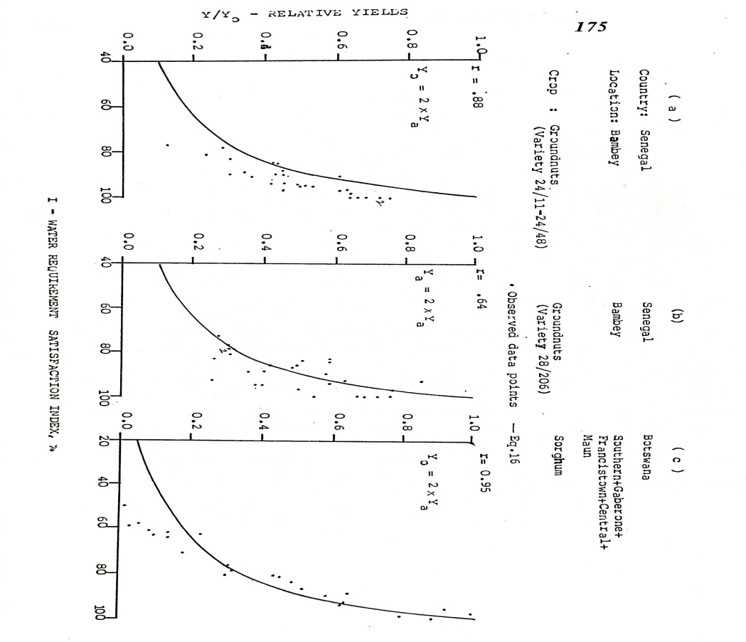
Figure 6: Comparison of crop yield function of Mozambique with the data of two groundnut varieties in the case of Senegal and sorghum data in the case of Botswana

4.Discussion:

The major issue here is the collection of detailed data on different parameters that form the inputs to the model. Then only the quality of predictions become near reality. The author carried out this task for Mozambique and Ethiopia. This facilitated to present food aid requirement for Ethiopia during 1989/90. Figure 7 presents the crop condition & drought condition in Mozambique during the crop season 1987/88 as explained in Table 2. At the end of this exercise checked the results with ground realities and found they are in line with the reality in field – Reddy & Daniel presented the summary and Recommendations [10 August 1988, Maputo, Mozambique] on “Special Crop Evaluation Mission’s Field Visit {during 21-30 June, 11-12 July & 26-30 July, 1988]”.

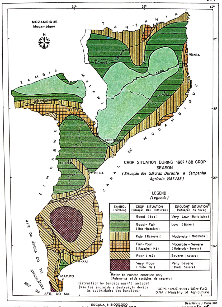
Figure 7: Crop condition during 1987-88 crop season: an example of Mozambique

Annexure-I:

Crop calendar along with decadal rainfall [R] and potential    evapotranspiration [PE] for 7 provinces in Mozambique

[A] Lichinga

[B] Ulongue

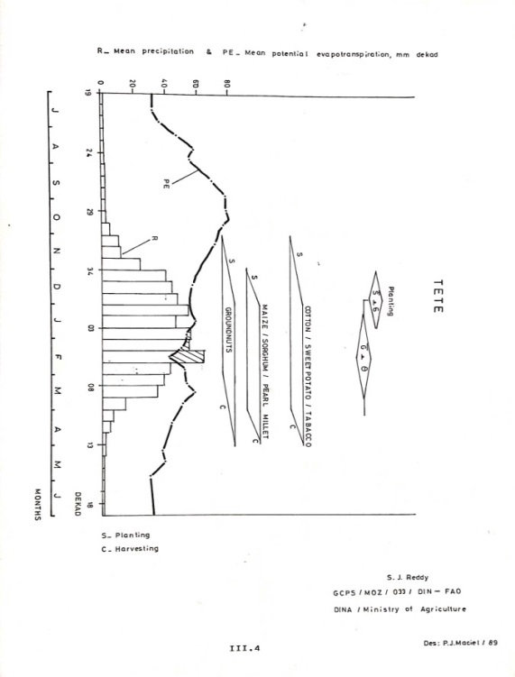
[C] Tete

[D] Nampula

[E] Quelimane

[F] Inhambane

[G] IAX-IAX

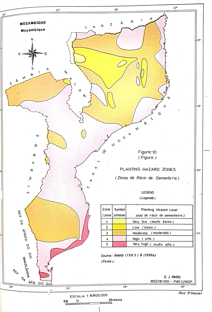
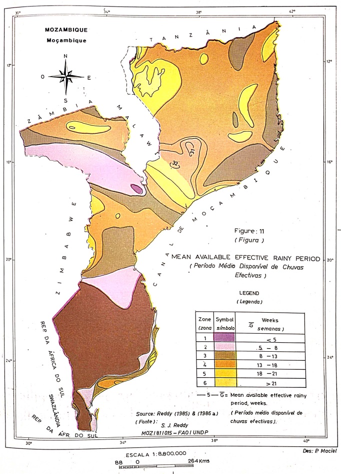
Annexure-II:

Generalized 8 Maps relating to terrain, soil, crop, climate of Mozambique

5.Summary & Conclusions:

1. The article discussed the method for the crop early warning and drought monitoring through agrometeological approach under family sector agriculture in developing countries;
2. This model takes into account soil, crop & weather;
3. The method was developed with reference to Mozambique and applied to Ethiopia;
4. In 1987/88 crops conditions were monitored throughout the crop season and issued bulletins at decade [ten day] interval. The bulletins were distributed to all government offices through the office of Agriculture Ministry and later through Prime Minister’s office in Maputo/Mozambique. At the end food aid requirements were presented for each province which was verified with ground realities and later FAO Food Aid Bulletin included this; and Respected President briefed the media.
5. In this article also proposed to improve the yield estimation by dividing the average yield data series according to natural variability or cyclic variations in rainfall, a main component of climate change;
6. However, this has no effect on drought index estimated for that year;
7. For state farms it is more appropriate to use different model [ICSWAB soil water balance model] – this was tested with Arkin’s SORGF model developed in A&M Texas under tropical semi-arid conditions.

Acknowledgement:

This research is self-funded. The author expresses his grateful thanks to those authors whose work was used for the continuity of the story. The author confirms that there is no conflict of interest involved with any parties in this research study