1.  Introduction:

For agriculture the two primary natural resources are land and water. The former is static, and the latter is dynamic resource. Most countries are placing unprecedented pressure on water resources with the fast-growing global population. Furthermore, chronic water scarcity, hydrological uncertainty, and extreme weather events (floods and droughts) are perceived as some of the biggest threats to global prosperity and stability. Acknowledgment of the role that water scarcity and drought are playing in aggravating fragility and conflict is increasing. Feeding 9 billion people by 2050 will require a 60% increase in agricultural production, (which consumes 70% of the resource today). Besides this increasing demand, the resource is already scarce in many parts of the world. Estimates indicate that 40% of the world population live in water scarce areas, and approximately ¼ of world’s GDP is exposed to this challenge. By 2025, about 1.8 billion people will be living in regions or countries with absolute water scarcity. Water security is a major – and often growing –challenge for many countries today. Natural rhythmic variations in rainfall play the pivotal role in dry-land or rain-fed agriculture as the source of water present changes with droughts and floods with the time. However, we remember the fact these statistics are hypothetical in nature. For example (i) we are have been wasting 40-50% of food and thus inputs used to produce that much food including water, and (ii) we are polluting water resources both surface and groundwater – though rain is unpolluted when it is used in agriculture under chemical inputs, plant get polluted water and thus food produced become polluted. 

It appears that people who harp on climate change has no basic knowledge on the subject “climate change” and its association with agriculture. Climate is dynamic,. Climate is always changing. Our fore-fathers adopted to such changes in climate and that knowledge passed it on to generations. Animal husbandry was part of it. That technology provided healthy diet, unpolluted air and water. In 60s this changed with the entry of multinational companies, now they are earning trillions of dollars each year,  wherein agriculture technology is based on chemical inputs tailored seed [hybrids, cultivars, GM] technology. This changed the food scenario. It is a polluted food technology [air, water & food]. This multifold increased the unhealthy population that in turn has been creating air, soil & water pollution. The UN is the major culprit in supporting this. They brought in the concept of global warming and green fund. Nations are running after this fund to get a share like fliies flock around sweeteners by wasting public money make honey-moon trips at COP meetings held around the world. It is a highly shameful. The only solution is to go back to our traditional agriculture system and population control.

Results are data dependent. Scientific community rarely account the natural variability in rainfall on water resources availability. They invariably use short period data series that don’t cover at least one cycle of natural variability. Therefore such data set will reflect biased  estimates. That means, these estimates don’t serve the needs of water resources planning and thus agriculture planning. Some other scientific groups use random periods as per the data availability for them. These give mis-leading or biased inferences/conclusions. The other important factor is soil. The soil water holding capacity defines the water resources availability in-situ for use in agriculture. The important issue is the selection of crops/cropping patterns.

A drought is an event of prolonged shortages in the water supply, it may be atmospheric (below-average precipitation), surface water or ground water. A drought can last for months or years. It can have a substantial impact on the ecosystem and agriculture of the affected region and harm to the local economy. Drought is a recurring feature of the climate in most parts of the world. However, these regular droughts present systematic variations in association with natural variability in climate, known as climate change. Though they are predictable, but they are beyond human control and thus needs to adapt to them.

There are three types of droughts in use, namely, meteorological, hydrological and agriculture. After the green revolution technology entered a fourth dimension, namely technological drought. All these are qualitative indexes. One can divide the effects of droughts and water shortages into three groups, namely environmental, economic and social. Effects vary according to vulnerability. For example, subsistence farmers are more likely to migrate during drought because they do not have alternative food-sources. Areas with populations that depend on water sources as a major food-source are more vulnerable to famine. Agriculturally, people can effectively mitigate much of the impact of drought through irrigation and crop rotation. Failure to develop adequate drought mitigation strategies carries a grave human cost in the modern era, exacerbated by ever-increasing population densities.  Dams and their associated reservoirs supply additional water in times of drought. However even the irrigation water primarily depends upon rainfall. Well-known historical droughts include:

1. 1540 Central Europe, said to be the “worst drought of the millennium” with eleven months without rain and temperatures of 5–7°C above the average of the 20th century
2. 1900 India killing between 250,000 and 3.25 million.
3. 1921–22 Soviet Union in which over 5 million perished from starvation due to drought.
4. 1928–30 Northwest China resulting in over 3 million deaths by famine.
5. 1936 and 1941 Sichuan Province China resulting in 5 million and 2.5 million deaths respectively.
6. The 1997–2009 Millennium Drought in Australia led to a water supply crisis across much of the country. As a result, many desalination plants were built for the first time (see list).
7. In 2006, Sichuan Province China experienced its worst drought in modern times with nearly 8 million people and over 7 million cattle facing water shortages.
8. 12-year drought that was devastating southwest Western Australia, southeast South Australia, Victoria and northern Tasmania was "very severe and without historical precedent".
9. 2015–2018 Cape Town water crisis. This likelihood was tripled by climate change. However, this is not a correct interpretation as this is part of natural change in rainfall.

This article discusses drought scenarios under different conditions including climate change.

2.Climate Change Scenario:

2.1. Global warming scenario:

IPCC’s AR6-WG-I Report:

On 9^th August 2021 released Intergovernmental Panel for Climate Change (IPCC) Working Group I report titled "Climate Change 2021: the Physical Science Basis", Though it is claimed that “The IPCC is the UN body for assessing the science related to climate change”, in reality it is not science of climate or the science of climate change but the study relates to a fictitious global warming and its impacts. Global warming of 1.5°C and 2.0°C will be exceeded during the 21st century unless deep reductions in CO₂ and other greenhouse gas emissions occur in the coming decades. This is the conclusion from the 1300 pages report, and this is a qualitative statement and not based on science. The entire issue runs around there is increasing greenhouse gases and they are contributing to rise in temperature. However, since 2000 they are struggling to get a scientifically defined value for “Climate Sensitivity Factor” that defines the link between greenhouse gases and temperature by following “trial and error” approach with no real solution.

The IPCC doesn’t tell governments what to do. Its goal is to provide the latest knowledge on climate change, its future risks and options for reducing the rate of warming. The IPCC doesn’t conduct its own climate-science research. Instead, it summarizes everyone else’s.  If this is so, where is the need to have a political body like IPCC, this can be executed by its parent scientific body, WMO, wherein all met services, who are more qualified in this area, in the World form part of it. Fundamentally Climate Change is “real” but not Global Warming, which is a fictitious value that serves the vested interest groups to collect 100 billion dollars per year up to five years to share under the disguise of Green Fund.

“IPCC report highlights how climate change is causing extreme events and exacerbating risks of floods and droughts” By Aditi Mukherji (IWMI), Aditi is a Principal Researcher at IWMI and is a Coordinating Lead Author of Water Chapter IPCC’s Working Group II, and a core writing team member of IPCC AR6 Synthesis Report.  Extreme weather events are increasing, and risks of floods and droughts are rising. In July, we saw catastrophic floods hit China, India and Europe. The ongoing famine caused by climate-induced drought in Madagascar has affected over a million people. More people than ever before are experiencing climate change daily, and much of that is experience through water related changes.  Are these extreme events linked to climate change, and are they increasing? Is climate change modifying the global water cycle? And what is causing climate change in the first place?  Extreme weather events are increasing, and risks of floods and droughts are rising.

The IPCC WGI Report, approved at the plenary session on August 9th, drilled down into these questions. These are our top eight takeaways on water and extreme events based on the report’s findings. Top eight takeaways on water and extreme events based on the report’s findings:

1. The WGI Report reiterates what we have now known for a while: those humans are driving a rise in temperature, thanks to carbon and other greenhouse gas emissions. Currently, the global surface temperature is around 1.09°C higher than in the pre-industrial period (1850-1900), with stronger warming over land (1.59°C) than over oceans. Several of the climate impacts are already observed at 1.09°C, and these impacts will intensify at higher temperature levels.
2. Every degree of global warming is likely to increase global mean precipitation by around 1% to 3%. A hotter planet is a wetter planet because a warmer climate increases the moisture content in the atmosphere and feeds into weather systems, making wet events wetter.
3. The frequency and intensity of heavy precipitation events of the kind we have recently seen in Germany and China have increased at a global scale. This is especially true for North America, Europe and Asia, where long term observational data exists. Every degree of global warming will further intensify such extreme precipitation events.
4. As extreme precipitation events increase, so too will the frequency and magnitude of surface water floods and flash floods. This is because when there’s high precipitation, the natural and artificial drainage systems cannot hold the excess water. As a result, a large amount of land is projected to be affected by river floods in the future, increasing with every degree of global warming.
5. A warmer, wetter world is also subject to increased evaporation leading to decreases in soil moisture and the likelihood of more droughts. For example, greater warming over the land surface reduces near-surface humidity on a continental scale, which contributes to drying at a regional scale. At 4°C of global warming, about 50 percent of all land areas will see increased frequency and severity of droughts. Even if global temperatures stabilize at an average increase of between 1.5°C to 2°C above pre-industrial levels, several regions, including South Asia, East, West and Southern Africa, will experience severe droughts. These also tend to be the places where a large majority of the poor people live and depend on rainfed agriculture for their livelihoods. Risks of forest fires also increase with temperature rise and droughts.
6. One of the most exciting scientific advances in the IPCC Sixth Assessment Report is the high confidence with which extreme event attribution to climate change has become possible. Almost all extreme events that we have witnessed in recent years have been made more likely due to climate change. On a global scale, climate change is now potentially detectable from any single day of weather data. However, at a more regional level, the lack of long-term data in certain geographies limits the possibility of extreme events detection and attribution.
7. Most perennial rivers, including the ten major rivers originating from the Hindu Kush Himalayas, that provide water and food security to large parts of Asia, are glacier-fed. Yet, glaciers are melting almost everywhere. According to the WGI report, from 2010 to 2019, glaciers lost more mass than at any time since glacier mass balance observations began. This trend is only likely to intensify with every degree of global warming and will have severe implications on river flows, livelihoods, energy production and cultural values.
8. How we use our land and grow our food has also influenced the hydrological cycle. For example, water extraction for irrigation has affected regional water cycles across some of the most intensively irrigated parts of the world, for example in South Asia. At the same time, large-scale deforestation is likely to lead to increased runoff, and urbanization has increased local precipitation and runoff intensity.

In summary, all components of the hydrological cycle have been impacted by human-induced climate change, and the way we use our land and water has, in turn, also intensified the impacts. Many people in developed and developing countries are experiencing extreme events. Furthermore, given the current projections for greenhouse gas emissions, it is likely that we are headed towards a 1.5°C world by the mid-2030s, where most of these impacts will intensify further. These are irrelevant and they are hypothetical-rhetoric statements of pro-global warming groups. 

2.2. Natural variability in rainfall: a case study:

The case of all-India rainfall:

The annual march of all-India average annual rainfall during 1871-72 to 2014-15 for June to May presented 60-year cycle. Two full 60-years cycles completed, and the third cycle started in 1987/88. The first 30 years represented above the average component of the cycle.  Mukund P. Rao, et al. published a study -- “Seven centuries of reconstructed Brahmaputra River discharge demonstrate underestimated high discharge and flood hazard frequency” in Nature communications  volume 11, Article number: 6017 (26^th November 2020): They used seven-centuries (1309–2004 C.E) tree-ring data for the reconstruction of monsoon season Brahmaputra discharge : According to this1957/58–1986/87  ranks amongst the driest of the past seven centuries (13th percentile)  -- this is the below the average 30 year period in All-India annual rainfall [1957/58-1986/87]; Also 1830-60 tree ring part of dry period fall under below the average 30 year period – this is below the average 30 year period in All-India annual rainfall  [1837/38-1866/67].  In Indian Parliament, members asked “Is Indian rainfall decreasing?” The government replied “yes”. This in fact is not correct. As we have seen from the above that Indian rainfall follows 60-year cycle. Government agencies used the data of 2^nd cycle wherein the first 30-year period is above the average and the next 30 years form below the average [1957/58-1986/87] and thus presented a decreasing trend. If they would have shifted 30 years backwords or forwards, then this would have given them increasing trend for the 60-year period. The frequency of occurrence of severe floods in north western India Rivers also followed this pattern. The yearly water flows in Godavari River during 1881 to 1946 [Bachawat Tribunal data set] followed 60-year cycle. Though the data presented 60-year period it presented zero trend as the centre 30-years form below the average and on either side of this above the average 30 years period are equally divided. That means data selection plays important role to get unbiased results and thus conclusions. Modern researchers invariably use truncated data sets due to several reasons without having the knowledge on such selections.

Case of Andhra Pradesh rainfall:

The annual march of Andhra Pradesh means annual rainfall [mean of the three met sub-divisions]; and the mean annual water availability in river Krishna followed the same 132-year cycle. For water sharing among riparian states two tribunals presented reports using different data sets as follows:

1. Bachawat Tribunal used 1894-95 to 1971-72 [78 years] water availability observed data of Krishna River. The mean of the data set is 2393 tmc ft. This is available at 43% probability level – negatively skewed data set;
2. Brijesh Kumar Tribunal used 1961-62 to 2007-08 [47 years] water availability observed data in Krishna River. The mean of the data set is 2578 tmc ft. This is available at 58% probability level – positively skewed data set;
3. For the combined data set of 1894-95 to 2007-08 (114 years], the mean is 2443 tmc ft available at 48% probability level – nearly normally distributed data set;
4. From Brijesh Kumar Tribunal 1981-82 to 2006-07 [26 years] data set presented a mean of 2400 tmc ft available at 50% probability level – normally distributed data set;
5. Central Water Commission [CWC] used 1985-86 to 2014-15 [30 years] data [estimated using a model].  The mean water availability estimate is 3144 tmc ft. This is available at 50% probability level – normally distributed data set [similar to the above 26 years data set];

The estimates must be unbiased, that means it should follow normal distribution, that means mean and median [50% probability] should coincide, that means on either side of the mean equal number of years must fall. In the above in the case of Bachawat  7 % values [50% - 43%]  are on lower side, that is biased towards lower values; and in the case of Brijesh Kumar it is 8% [58%-50%],on upper side, that is biased towards higher values; and thus they are termed as negatively Skewed and positively Skewed data sets, respectively.  Thus, the means are presented respectively lower [2393 tmc ft] and higher [2578 tmc ft] values. By joining the two data series it is nearly normal [50% - 48%] and even the short period of 26 years data set also present normal distribution. Both showed nearly the same means [2443 tmc ft and 2400 tmc ft]. CWC used 30 years data set.  However the 30 year period also followed normal distribution similar to 26-years data set but CWC mean is nearly 30% higher than that as the method used for the estimation of water flow in the river present overestimates as the model under estimates evapotranspiration and thus runoff presents the overestimate; however the other four data sets are observed flows. [see for more details: Reddy (2016, 2019, 2021a, b & c and 2022a)].

2.3. Selection of data scenario:

It is clear from the above sub-section that selection of data series play an important role if the data series that follows rhythmic or cyclic variation. Some such scenarios are discussed with reference to rainfall data selection at all India level and Andhra Pradesh state level. For example, Central Water Commission used the rainfall data of 30-years [1985-86 to 2014-15] for the estimation of water availability in Indian rivers. They argued that IMD using 30 years for computation of climatic normals of met parameters. They have no knowledge on this concept of IMD. WMO proposed this for inter-comparison of data of the world and regions in a country. At the same time it is not fixed. The period changes as time progresses. For example, first the met services prepared normal books for their countries using the data of 1931-60. Later this was for 1961-90. Next will be for 1991-2020.  WMO (1966) discussed this issue of selection of data series.

3. Case studies of drought scenarios:

Discussed four scenarios namely, agroclimatic variables, natural variability impact on agroclimatic variables, climate interaction with the soils; and climate interaction with the soils and the crops. These are explained with few examples.

3.1. Agroclimatic variables:

Input data: weekly rainfall [R] and potential evapotranspiration [PE];

Methodology:

Reddy (1983a & 1993) presented a method of estimation of agroclimatic variables. The following 5 agroclimatic variables are derived from R & PE using 14-week moving averages of R/PE technique:

G         =          Available effective rainy period

S          =          the week before the commencement of G is taken as the week

of commencement of sowing rains;

W        =          the number of weeks within G wherein R/PE ≥ 1.5, which is termed

as wet period

D         =          the number of weeks within G wherein R/PE ≤ 0.50, which is termed

as dry period

The averages of these four parameters for N years are computed.

A         =          the percentage number of years for which G ≤ 5 weeks, which

is termed as drought proneness of the location.

Figure 1a presents the distribution of “A”, the drought proneness map of India. Figure 1b the same for Maharashtra State in India [Akumunchi Anand et al., 2009]. In both the figures the impact of Western Ghats [rainfall shadow zone] on A is clearly seen. Reddy (1993) presented such maps for few countries including Mozambique.

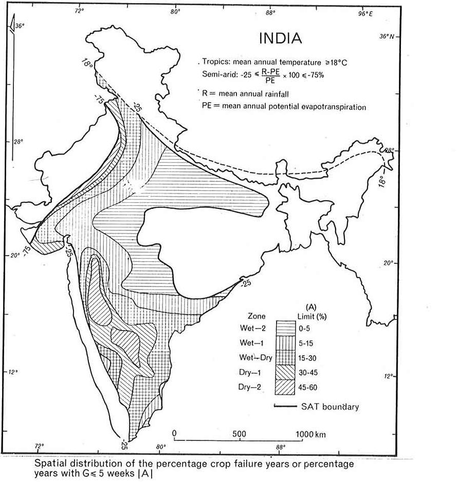
Figure 1a: Agroclimate based drought prone map of India

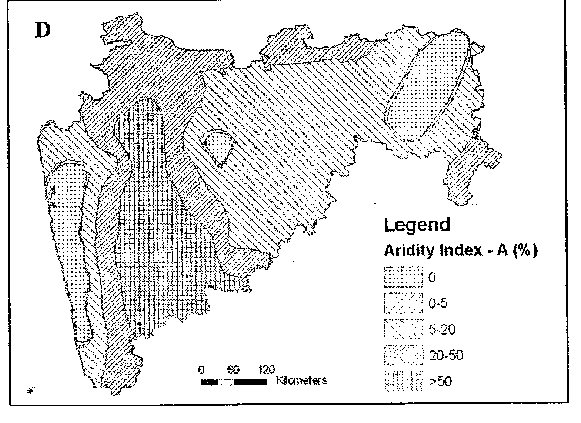
Figure 1b: Agroclimate based drought prone map of Maharashtra

3.2. Natural variability impact on agroclimatic variables:

Rainfall presents the natural variability around the world (Reddy, 2000, 1981, 1984b, 1986, 1993) -- in India, Brazil, Mozambique, Botswana & South Africa; and Reddy & Mersha (1990) in Ethiopia.

Agroclimatic variables G & S were computed for Kurnool in Andhra Pradesh India. The annual march of G & S is presented in Figure 2. Reddy (2000) observed 56-year cycle in southwest monsoon rainfall of Rayalaseema [as well Coastal Andhra & Telangana] met sub-division. This 56-year cycle is supposed In Figure 2. The table in the figure presents averages of G and S for the segments of below and above the average parts of 56-year cycle. This analysis presented A = 45% of the years for Kurnool; and the same for below and above the average periods are 70% and 30%, respectively. This gives ample evidence on the importance of sub-division of data series according natural variability [if any] to get better results on possible agriculture scenario.

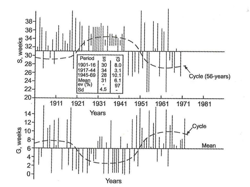
Figure 2: Agroclimatic variables versus natural variability for Kurnool in Andhra Pradesh

3.3. Climate interaction with the soil:

Input data:

R         =          daily rainfall, mm

E          =          daily open pan US Class “A” evaporation with mesh cover, mm

 

Methodology:
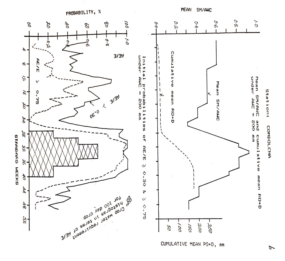
Williams, et al. (1985) discussed the role of soils in climate analysis. Using the ICSWAB soil water balance model (Reddy, 1983a) simulations under different soil types were carried out (Reddy, 1993) and presented in Figure 3 for Combolcha in Ethiopia.

Results:

For the analysis N years’ data of R & E were used. The analysis was carried out for three soil and two crop conditions, namely, (a) Alfisols (AWC = 100 mm); (b) Vertisols (AWC = 200 mm) with 100-day crop and (c) under Vertisols with intercropping (100/180 days). AWC is the soil water holding capacity of the soils in mm.

Using this data of N years estimated actual evapotranspiration (AE) in mm, soil moisture reserve (SM) in mm and surface runoff + deep drainage (RO+D) in mm at weekly interval and then estimated AE/E & SM/AWC. 

Using this data at weekly interval [standard weeks] estimated probability values of AE/E ≥ 0.30 and ≥ 0.75 and are shown in Figure 3 [lower part]. These figures also present the crop water requirement histograms in terms of AE/E for a 100-day crop or 100/180-day intercrops [hatched area]. This histogram was constructed with the following threshold limits:

AE/E ≥ 0.30                represents the limit for initial growth of a dry-land crop and/or pastures;

AE/E ≥ 0.60                represents the limit for optimum growth of pastures;

AE/E ≥ 0.75                represents the optimum limit for dry-land crops;

The crop water requirements are met in about 85 and 95% of the years, respectively in Alfisols and Vertisols, with week no. 27 as the planting week. 

In Figure 3 [a & b] the upper part includes the mean of SM/AWC and cumulative mean of (RO+D). At the harvest of the 100 day crop the average relative soil moisture reserve [SM/AWC] is expected to be 60% and 70% of AWC in Alfisols and Vertisols, respectively. In Vertisols [Figure 3c] intercropping of 100/180 days presents the similar results.

It is clear that the 1^st rainy season is not suitable for a dry-land crop, but short-duration legume pasture can be practiced to protect the soil and thereby increase soil potential. The mean cumulative runoff on Alfisols and Vertisols respectively is about 200 and 150 mm, of which 60% is expected to go as surface runoff and 40% as deep drainage, mostly occurring in week no.27-39.

Table 1 presents probabilities of crops having fully adequate soil moisture regime for 90-day kharif crop on Vertisols of three areas, namely Sholapur, Hyderabad and Akola.  In the case of example in Table 2 climate [three locations] and soils AWC [230 & 120 mm]. Column 7 in the table shows the total probability of a 90-day kharif crop encountering good growth conditions throughout the growth period; column 8 presents probability of adequate moisture for rabi sorghum after kharif crop; and column 9 presents probability of adequate soil moisture after kharif fallow. Table 2 presents success of different crops in rainy & post-rainy seasons at four stations, namely:  Sholapur [Vertisols with AWC = 250 mm], Hyderabad Alfisols with AWC = 125 mm & Vertisols with AWC = 250 mm], Akola [Alfisols with AWC = 175 mm & Vertisols with 250 mm] & Indore [Vertisols with AWC = 250 mm]. AWC is the water holding capacity of the soils [K]. Here all the three parameters showed change – soil, climate & crop.

[a]

[b]

[c]

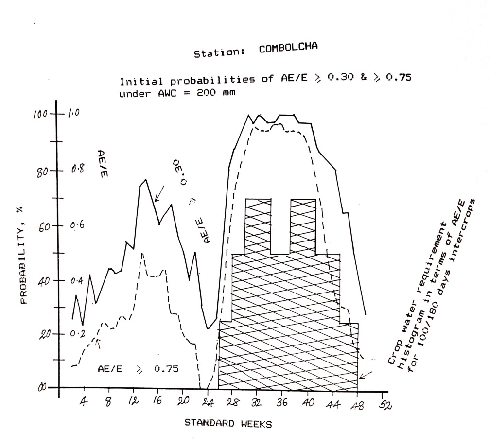
Figure 3: Probabilities of soil water balance parameters for Combolcha in Ethiopia under (a) Alfisols (AWC = 100 mm); (b) Vertisols (AWC = 200 mm) with 100-day crop and (c) under Vertisols with intercropping (100/180 days) – Source: Reddy (1993)

For example, the successes of different cropping patterns on seasonal basis for Hyderabad are:  In both Alfisols and Vertisols, a 91-day kharif crop is successful in 56% of the years in Vertisols and 27% of years in Alfisols. In around 43% and 36% of the years there is a possibility of receiving rains more than 50 mm at harvest maturity. For a 105-day kharif crop, success is the same as that of a 91-day crop, but the success of a 100-day rabi crop is reduced substantially, to 13 and 36% for Alfisols and Vertisols, respectively. An intercrop of 91/180 days is successful in 83 and 90% of the years under Alfisols and Vertisols, respectively. This is the best cropping pattern for the Hyderabad region under both soil types. However, with good early rains, a sequential crop is also possible for Vertisols.  Same way the other stations can be explained. 

The output of Figure 3 and Tables 1 & 2 are based on ICSWAB model (Reddy, 1983a) using daily rainfall data...

Table 1: Reliability of a 90-day kharif crop on Vertisols of three areas (probabilities expressed in percent of years] – Source: Binswanger, etc. al. (1980)

Duration of crop	Percentage success of different duration crops
	Sholapur	Hyderabad			Akola			Indoreb
(days)	1	2		1	3	1		1*
(a) Rainy season crop
70a	75	--		--	--	--		--
70b	17	--		--	--	--		--
91a	58	91		91	100	100		100
91b	25	36		43	22	28		62
105a	58	91		91	100		100	100
105b	11	17		41	19		14	43
119a	--	80		90	94		97	100
119b	--	4		30	00		03	00
(b) Intercropping
91/180	78	83		90	81	83		97
(c) Double croppingd
70 + 100	81	--		--	--	--		--
91+ 100	81	27		56	33	42		81
105 + 100	67 19		13	36	14			51

Table 2: Success of different crops in rainy & post-rainy seasons at four stations^a

           

* 1 = Vertisols (K = 250 mm), 2 = Alfisols (K = 125 mm), 3 = Alfisols (K = 175 mm)

a = percentage number of years for successful kharif crop

b = percentage number of years in which rains of more than 50 mm occurred at harvest maturity

^a: Source: Reddy (1984a)

^b: 40% of the years represent a problem for interculture

^c: 91/180 refers to an early maturing variety of 91 days and a late maturing variety of 180 days [for example, a 91-day sorghum and 180-day pigeonpea]

^d: 70 + 100 refers to a 70-day rainy season crop followed by 100-day post-rainy season crop (for example, a 70-day cowpea followed by 100-day sorghum

3.4. Climate interactions with the soils and with the crops:

FAO Model:

Here water balance was carried out using FAO model [FAO, 1986]. The drought index was 64, 74 & 86% respectively for the three soils with water holding capacities – 60, 100 & 150 mm  under maize crop during 1989 at Yabelo in Ethiopia at the harvest (Reddy, 1991) -- see  Table 2 of Part-II (Reddy, 2022b) for the details on the computation procedure.

ICSWAB Model:

ICRISAT scientists collected experimental data on sorghum [grain yield and total biomass] over wide range of soils and climate conditions and tried to test the SORGF model of Arkin, et al. (1976) developed at AM Texas in USA. The field data includes both kharif and rabi seasons for years 1979 and 1980 for five sorghum cultivars [CSH1, CSH6, CSH8, M-35-1 and SVP-351]. SORGF ability to predict grain yield and dry matter for 23 data sets was carried out. They observed that the root means square errors [RMS] and correlation [r] for dry matter and grain yields were 27.58 and 17.39 q/ha; and 0.35 and 0.37, respectively. This is based on Ritchie (1972) soil water balance model which works under conserved soil moisture conditions. Even after changing the energy factor in the model, there was no improvement in the RMS and r.

ICRISAT Director General in the workshop asked me to present the results by changing the soil water balance output with my model [ICSWAB].  I presented the soil water balance output from ICSWAB model. By replacing the Ritchie’s model output with ICSWAB model output, the corresponding values for RMS were 15.06 and 8.49 q/ha, and r were 0.85 and 0.81 (Reddy, 1984a).  That is, appropriate model selection plays important role in getting reliable results. SORGF model worked very well where it was developed but failed under rainfed condition. ICSWAB model was developed to account conserved soil moisture condition and as well under daily rainfall conditions. However, Arkin refused to change his model structure and as a result ICRISAT Scientists closed the research with that model.

4.Summary & Conclusions:

1. There are three types of droughts in use, namely, meteorological, hydrological and agriculture. After the green revolution technology into agriculture, entered a fourth dimension, namely technological drought. All these are qualitative indexes;
2. To get unbiased estimates there are several scenarios, namely: data selection & models’ selection to estimate drought; 
3. The representativeness of drought index relates to the selection of rainfall data set. The rainfall data set must follow the normal distribution. If they are skewed distributions [positively or negatively] the resulting index will be biased towards higher or lower values;
4.  In the case of drought assessment, four scenarios are discussed, namely agroclimatic variables based, the impact of natural variability on climatic variables based, soil-water based & soil-water-crop based – details on the last one is presented in Part-II of the article;

That is for assessing agriculture related drought should be based on crop, soil and water. Individually these parameters may present different drought conditions that may help in assessing long term agriculture planning. The integrated index helps in early warning of crop scenarios – see Part II. The impact of natural variability in rainfall on agroclimatic variables scenarios helps long term agriculture planning. The same is the case with climate and soils scenarios.

This is the reality of the Science!!!:

Acknowledgements:

The research is self-funded. The author expresses his grateful thanks to those authors whose work was used for the continuation of the story. The author also confirms there is no conflict of interest involve with any parties in this research study.