Agricultural Research Pesticides and Biofertilizers
OPEN ACCESS | Volume 6 - Issue 1 - 2026
ISSN No: 2994-0109 | Journal DOI: 10.61148/2994-0109/ARPB


Navneet Raj Rathore 1*, Anurag Gupta 2, R. B. Singh 3
1AKS University, Satna, M.P.
2School of Studies in Statistics, Vikram University, Ujjain (M.P.)
3Department of Mathematics & Statistics College of Agriculture, JNKVV, Jabalpur (M.P)
*Corresponding Author: Navneet Raj Rathore, AKS University, Satna, M.P.
Received: July 28, 2021
Accepted: August 05, 2021
Published: August 10, 2021
Citation: Navneet Raj Rathore , Anurag Gupta and R. B. Singh . (2021) “Fitting Statistical Model to Some Agricultural Dynamic Variables Maize (Zea Mays) Production and Productivity in Betul District.”, Journal of Agricultural Research Pesticides and Biofertilizers, 2(3); DOI:http;//doi.org/07.2021/1.1038
Copyright: © 2021 Navneet Raj Rathore. This is an open access article distributed under the Creative Commons Attribution License, which permits unrestricted use, distribution, and reproduction in any medium, provided the original work is properly cited.
For the Betul District, stochastic models for maize production and productivity were fitted in this work. Linear model, Quadratic model, Compound model, Cubic model, and Power stochastic models were used. We utilised different comparison metrics to assess model fitting performance like R2, adjusted R2 and residual mean squared error. According to the findings, the compound and power models are the best at forecasting all of the important elements in Betul District.
Introduction:
Using the correlation & path analysis approach, this study identifies the noteworthy factors impacting maize output in Betul District and Madhya Pradesh as a whole. The region has the greatest direct influence on total maize output, whereas the price of maize has the greatest indirect influence. It shows that as the size of the region grows, so does productivity.
The comparison criteria like R2, adjusted R2 and residual mean squared error (RMSEE), compound and power are the best suited model for predicting for the crucial two elements production and productivity in the current study. Singh (2013) utilised a similar model fitting method and concluded that compound and power are the best statistical models based on different goodness of fit criteria. Betul, a maize crop, is one of the most significant Cereals crops in Madhya Pradesh, providing 6.0 percent. From 1988 to 2017, the area, production, and productivity all increased at a positive pace for 30 years in a row During the time, expanding the area, production, and productivity of maize shall be done by increasing the area, production, and productivity by 6.30 percent, production by 8.90 percent, and productivity by 2.60 percent.
Madhya Pradesh is the largest producer, accounting for 5.7 percent of national maize production, and similar areas, production, and productivity have all grown at a positive rate, with area increasing by 1.0 percent, production increasing by 2.70 percent, and productivity increasing by 1.70 percent during the period. Statistical methods and procedures should be utilised to correctly assess the scope of growth in order to attain this aim. I expect that the findings of the proposed research would be useful to farmers and researchers in determining or increasing the trend of area, production, productivity, price of maize crop and fertiliser distribution pattern in Betul District and Madhya Pradesh State.
Materials and Methods:
For the objective of the project, data on five essential parameters linked to maize will be collected for the Betul District. For 30 years, data from the Directorate of Economics and Statistics and M.P.Krishi.org will be collected (1988 to 2017).
Statistical Model Fitting:
The above-mentioned models' functional form is 
where,  is the Maize output / productivity in the ith year,
  is unknown parameter to be estimated, P is Parameter and ɛt is random error i.e. ɛt’ s~ i.i.d. N (0, σ2).
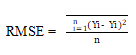
The five models were fitted on the data of year wise, one year at a time, up to the 30 year, which was the final step. These models' functional for RMSE are as follows:
where, Y t = response of the i-th factor in the tth year
α, β = unknown parameter, to be estimated, of the model, α (constant).
εt = multiplicative error
The linear models' parameters were calculated using the ordinary least squares (OLS) approach. The parameters of nonlinear models with multiplicative error terms were linearized using appropriate transformations, and the model parameters were estimated using the OLS approach.
These models are also stable when it comes to forecasting future values for each component. On the basis of the parameters R2, RMSE, and Adjusted R2 values, the results obtained after fitting various models were compared. On the basis of available data, the model with the lowest mean squared error and greatest R2 was deemed the best for that particular factor.
For model validation, the following parameter was used:
In order to establish the model's validity as a dynamic system, its stability and capability to stimulate historical data were studied. The model's performance was evaluated using the coefficient of determination (R2), residual mean squared error, and adjusted R2.
1. Coefficient of determination:
The coefficient of determination is used to assess the goodness of fit.

2. Residual variance:
The lower the RMSE number, the better the model.
3. Adjusted R2:
The change in R2 that changes the number of words in a model is known as adjusted R2. The proportion of the variance in the dependent variable accounted for by the explanatory factors is calculated using the adjusted R2.
The Adjusted R2 defined as:

where k is the number of model parameters including the intercept term.
Separately, the aforesaid criteria were applied to data sets on production statistics relevant to the issues under investigation. The OLS method was used to estimate the parameters of these models. Fitted improved models were largely checked and evaluated for their suitability in terms of error characteristics by critically comparing and assessing parameter estimates, summary statistics, such as coefficient of determination R2; residual mean squares (RMSE) or error variance, and Adjusted R2 values. A best fitted parsimonious model has the least RMSE with the fewest parameters among a collection of competing best fitted appropriate models.
|
Year |
Maize Production X2 (000 tons) Betul District |
Maize Productivity X3 (ton/ha.) Betul District |
|
1988 |
10.4 |
0.965 |
|
1989 |
12.4 |
1.020 |
|
1990 |
13.3 |
1.137 |
|
1991 |
13.2 |
1.025 |
|
1992 |
13.4 |
0.980 |
|
1993 |
16.5 |
0.995 |
|
1994 |
15.1 |
1.025 |
|
1995 |
13.4 |
1.075 |
|
1996 |
19.7 |
1.112 |
|
1997 |
23.1 |
1.185 |
|
1998 |
22.7 |
1.242 |
|
1999 |
30.5 |
1.433 |
|
2000 |
39.4 |
1.789 |
|
2001 |
72.9 |
2.882 |
|
2002 |
60.5 |
2.273 |
|
2003 |
71.3 |
2.221 |
|
2004 |
85.1 |
2.017 |
|
2005 |
72.0 |
1.618 |
|
2006 |
72.0 |
1.597 |
|
2007 |
50.6 |
1.054 |
|
2008 |
63.5 |
1.373 |
|
2009 |
59.8 |
1.406 |
|
2010 |
59.0 |
1.267 |
|
2011 |
75.8 |
1.563 |
|
2012 |
72.0 |
1.456 |
|
2013 |
176 |
3.500 |
|
2014 |
59.2 |
1.115 |
|
2015 |
43 |
2.389 |
|
2016 |
133 |
2.229 |
|
2017 |
179 |
2.400 |
Table1: Total Maize Production and Maize Productivity (Yield) of Betul District in the past.
Source: The data gathered from the Directorate of Economics and Statistics, M.P.Krishi.org (1988-2017).
|
Models |
t = 26 |
t = 27 |
t = 28 |
t =29 |
t = 30 |
|
|
R2(%) RMSE Adjusted R2 |
R2(%) RMSE Adjusted R2 |
R2(%) RMSE Adjusted R2 |
R2(%) RMSE Adjusted R2 |
R2(%) RMSE Adjusted R2 |
||
|
Linear |
67.10 467.69 0.657 |
62.80 508.56 0.614 |
55.10 591.82 0.533 |
59.60 618.13 0.581 |
62.00 776.93 0.606 |
|
|
Quadratic |
68.90 460.95 0.662 |
63.00 527.89 0.599 |
55.70 606.47 0.522 |
59.60 641.89 0.564 |
63.40 774.96 0.607 |
|
|
Cubic |
69.20 476.94 0.650 |
63.50 543.70 0.587 |
59.30 580.70 0.542 |
59.90 661.15 0.551 |
64.00 791.26 0.599 |
|
|
Compound |
85.70 0.097 0.851 |
82.60 0.115 0.819 |
76.30 0.151 0.753 |
78.30 0.145 0.775 |
80.40 0.143 0.797 |
|
|
Power |
75.80 0.163 0.748 |
75.80 0.160 0.748 |
73.80 0.166 0.728 |
74.60 0.170 0.737 |
74.80 0.184 0.739 |
Table:2 The impact of several criteria (model-by-model) on overall maize output in the Betul District.
For maize production in Betul District, the best fitting models with parameter R2, RMSE, and Adjusted R2 are compound, power, and quadratic. In 2013, the value of the compound model with parameters R2, RMSE, and Adjusted R2 was 85.7 percent, 0.97, 0.851, and in 2014, the value of R2, RMSE, Adjusted R2 was 82.6 percent, 0.115, 0.819, and the value of R2, RMSE, Adjusted R2 was 82.6 percent, 0.115, 0.819. In 2015, adjusted R2 was 76.3 percent, 0.151, 0.753, and the value of R2, RMSE, In 2016, adjusted R2 was 78.3 percent, 0.145, 0.775, and the value of R2, RMSE, In 2017, the adjusted R2 was 80.4 percent, 0.143, and 0.797.
The value of power model with parameter R2, RMSE, and Adjusted R2 is 75.8%, 0.163, 0.748 in year 2013 and the value of R2, RMSE, Adjusted R2 in 2014 is 75.8%, 0.160, 0.748 and value of R2, RMSE, Adjusted R2 in 2015 is 73.8%, 0.166, 0.728 and value of R2, RMSE, Adjusted R2 in 2016 is 74.6%, 0.170, 0.737 and value of R2, RMSE, Adjusted R2 in 2017 is 74.8%, 0.184, 0.739.
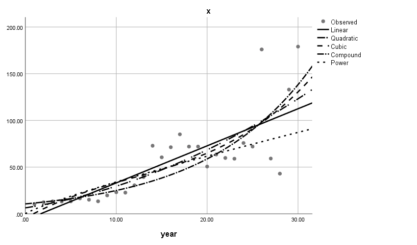
Graph 1: Diagram showing the fitting of maize production in Betul District.
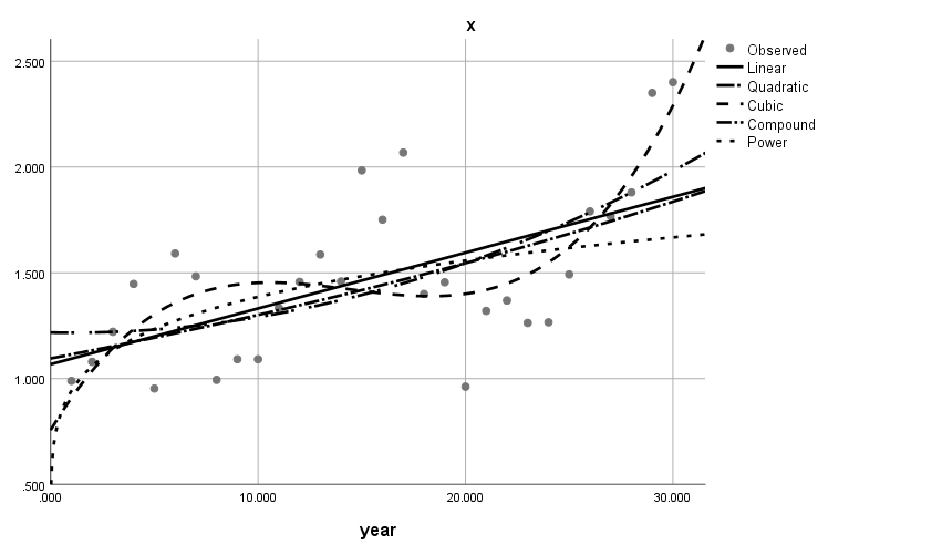
Graph 1: Diagram showing the fitting of maize Productivity in Betul District.
|
Models |
t = 26 |
t = 27 |
t = 28 |
t =29 |
t = 30 |
|
|
R2(%) RMSE Adjusted R2 |
R2(%) RMSE Adjusted R2 |
R2(%) RMSE Adjusted R2 |
R2(%) RMSE Adjusted R2 |
R2(%) RMSE Adjusted R2 |
||
|
Linear |
13.00 0.082 0.094 |
16.90 0.080 0.136 |
21.80 0.079 0.188 |
29.30 0.091 0.267 |
35.90 0.100 0.336 |
|
|
Quadratic |
19.90 0.078 0.129 |
20.20 0.080 0.135 |
22.70 0.081 0.165 |
29.60 0.094 0.242 |
38.40 0.099 0.339 |
|
|
Cubic |
20.20 0.082 0.093 |
22.50 0.081 0.124 |
27.90 0.079 0.188 |
41.00 0.082 0.339 |
52.50 0.080 0.470 |
|
|
Compound |
14.40 0.041 0.109 |
18.20 0.040 0.149 |
22.70 0.040 0.197 |
29.40 0.042 0.268 |
35.50 0.043 0.332 |
|
|
Power |
19.90 0.039 0.166 |
22.50 0.038 0.194 |
25.40 0.038 0.225 |
53.40 0.042 0.259 |
31.50 0.046 0.290 |
Table 3: The impact of several criteria (model-by-model) on maize productivity in Betul District.
In 2013, the value of a quadratic model with parameter R2, RMSE, and Adjusted R2 was 68.9%, 460.95, 0.662, and in 2014, the value of R2, RMSE, Adjusted R2 was 63.0%, 527.89, 0.599, and in 2015, the value of R2, RMSE, Adjusted R2 was 55.7 percent, 606.47, 0.522, and in 2016, the value of R2 ( Table 4.9).
Compound, power, and quadratic models are determined to be the best fitting models for maize production in Betul District when parameter R2, RMSE, and Adjusted R2 are taken into account. In 2013, the value of the compound model with parameter R2, RMSE, and Adjusted R2 was 14.4%,.041, 0.109, and in 2014, the value of R2, RMSE, Adjusted R2 was 18.2%, 0.040, 0.149, and in 2015, the value of R2, RMSE, Adjusted R2 was 22.7 percent,0.040,0.197. In 2016, the value of R2, RMSE, Adjusted R2 was 29.4 percent, 0.042, 0.268, In 2017, R2, RMSE, Adjusted R2 was 35.5 percent, 0.043, 0.268, respectively. The value of power model with parameter R2, RMSE, and Adjusted R2 is 19.9%, 0.039, 0.166 in year 2013 and the value of R2, RMSE, Adjusted R2 in year 2014 is 22.5%, 0.038, 0.194 and value of R2, RMSE, Adjusted R2 in 2015 is 25.4%, 0.038, 0.225 and value of R2, RMSE, Adjusted R2 in 2016 is 53.4%,0.042, 0.259, in 2017, the value of R2, RMSE, and Adjusted R2 was 31.5 percent, 0.046, 0.290. In the year 2013, the value of the quadratic model with parameter R2, RMSE, and Adjusted R2 was 19.9%, 0.078, 0.129, and the value of R2, RMSE, Adjusted R2 in 2014 was 20.2 percent, 0.080,0.135, and the value of R2, RMSE, Adjusted R2 in 2015 was 22.7 percent, 0.081, 0.165, and the value of R2, RMSE, Adjusted R2 in 2016 was (Table 4.10).

Open Access By Aditum Open Access Journals id licensed under Creative Commons Attribution 4.0 International License. Based On a Work at aditum.org