1. Introduction:

Plantbreeding is tied with the ancient plant characteristics improvements for human uses. The exact time of beginning is not well known, but domestication and selection were begun at the era of hunting and gathering. It was the symptom of pre traditional art of breeding and base for the latest desired current and future breeding. Hence, easily defining the “plant breeding” which constructed from two words is complex.

Plant breeding is the science, art, and business of changing plant genetics to produce desired traits in which indicated the interests of plant breeder specific to the society’s preferences(Hartung and Schiemann, 2014). Basic concepts of breeding will be developed new cultivar from existed genotypes in existed environments. It takes time and combination of different material and synergism of organizations to be achieved e.g. plant material, skilled human power, favorable working environments and takes time or process.  However, in the way of application, considerable challenges faced plant breeders. The interaction of genotypes within different environments which might positive or negative result taken as an example.

A cultivar grown in different environments frequently show a significant fluctuation in at least any of growth performance relative to other cultivars. These changes are influenced by the different environmental conditions are referred to as genotypes environmental interaction (GEI) (Dos et al., 2003). Phenotypic performance of a cultivar is the accumulation effect of the gene, environmental and their interaction.

Plant breeding in multi-environmental trials could be important to test general and specific cultivar adaptation.  Separate estimation of each source of variation may be complex and it takes time to decide.  For a long period of time, scientists and different stake holders tried to verify GEI different model. Most of the model on the market were described separately each of the sources as main and provided as cumulative effects in the residues of their multiplicative effect.

Several techniques of analyzes model have been developed to identify the major and interaction effects of genotypes and environmental factors. Analysis of variances (ANOVA), linear regression, and principal component analysis (PCA), GGE by plots and Additive main effect and multiplicative Interaction (AMMI) models used to study GE interaction in plant breeding.

Additive main and multiplicative model (AMMI) is more appropriate in GEI and important model to analysis, specially, when interaction between the environment and the genotypes provide significant(Zobel et al., 1988; Gauch and Zobel, 1996).  It is the summary of the various statistical model used for analyzing GEI.

AMMI is describes in one table compiled summary of analysis of variance (ANOVA), linear regression, and PCA of the genotypes by environmental interaction to check genotypes stability data(Zobel et al., 1988). AMMI is important to describe separately additive main effects in the experiment, which Genotypes and environment, each effect in the residual than definite provided error. To increase accuracy, it is the primary important model when main effects and interaction are both important (Zobel et al., 1988). It has the capacity to identify the impacts of genotype and environment in the interaction.

2. Methods of the study:

The study was followed around the desk research methods.  The sources of information were harvested online from the internet. The document related with AMMI model and have information were downloaded through google scholar application. Those documents were carefully read and relevant information to the outline were sorted out and paraphrased in to develop the paper. The over locations data were analyzed by AMMI using scripts of R software version of 4.1.

3. Concepts of AMMI:

The initial idea of AMMI was started in half of the twenty centuries by the work of different scientists which provided a substantial contribution to the development of the AMMI models (Williams,1952;Gollob, 1968; Mandel, 1971; Bradu and Gabriel, 1978).However, the application of the AMMI model in agricultural research was proposed by the study of Kempton in 1988 and Zobel et al 1988. Now, it is used in agricultural GEI experiments and most frequently recommended and usable at a condition where interaction is significance.

Various studies were tried to define additive main effect and multiplicative inter­action (AMMI) models and its tenacities. AMMI uses for analysis of vari­ance to study the main effects of genotypes and envi­ronments and principal component analysis for the residual multiplicative interaction among genotypes and environments(Silveira et al., 2013). The AMMI method integrates analysis of variance (ANOVA) and principal component analysis (PCA) into a unified approach that can be used to analyses multi-location trials (Zobel et al., 1988; Crossa et al., 1990; Gauch and Zobel, 1996). 

The AMMI classified total sum of squares (SS) of traits of interest partitioned into three general sources: the genotype main effect, the environment main effect, and the genotype X environment (GE) interaction (Zobel et al.,1988). Both of Genotypes and Environments (main effects) are additives, and interaction (residual from the additive model) non additive (Snedecor and Cochran,1980). Commonly, all three sources included in AMMI under GEI are statistically significant and agronomically important at condition where interaction significant (Kempton, 1984; Freeman, 1985).

Different routines statistical analysis models were applied to analysis yield or agronomic data collected over different environments and genotypes. The major statistical tool used to analysis were, Analysis of variance (ANOVA), principal component analysis (PCA) and linier regression (LR) analysis (Zobel et al., 1988). However, some important weaknesses were interlinked with the tools. 

The first, Analysis of variance (ANOVA) was provided only Additive effects of the variances which included genotypic and environmental effects effectively (Snedecor and Cochran, 1980). It has provided other sources of variances as undefined residues.  ANOVA can test the significance of the GE interaction, but this test may prove to be misleading. In any case, ANOVA provides no insight into the individual patterns of genotypes or environments that give rise to the interaction (Zobel et al., 1988).

The second statistical tool use to analysis over different environmental location was linear regression analysis.  Linear regression models combine additive and multiplicative components and thus analyze the main effects and the interaction (Mandel, 1961). There are several deficiencies in the fitting procedure of the most commonly used model (Finlay and Wilkinson, 1963). It was since the staged to fit the interaction component is known not to give theleast-square fit (Gabriel, 1978). Additionally, the LR model, in general, misperceives the interaction with the main effects, reducing its power for general significance testing (Wright, 1971).The third often used and flexible in GEI studies was Principal component analysis (PCA). It is analysis only the multiplicative parts. Principal components analysis, a multiplicative model, has the opposite problem of not describing the additive main effects (Zobel et al., 1988). The residual from the additive model is not even considered, except multiplicative or the interaction only.

Analysis of variances (ANOVA) provided nonsignificance where a  data collected from GEI due to the model problems, however more appropriate statistical model may both detect significance and describe interesting patterns in the interaction(Zobel et al., 1988).  This problem arises because the interaction contains a large number of degrees of freedom (G- 1) X (E- 1) G is genotypes and E represent a number of environments degree of freedom (Zobel et al., 1988). As a result, near to 50 % of SS where partitioned which make equal or less than mean square of interaction with the mean square of error, hence be declared insignificant by an F-test. AMMI is a model developed considered those problems.

3.1.  Prior model of GEI and its description:

Before the development of the AMMI model, several models were developed to analysis fairly the additive and multiplicative parts expected in GEI studies. The simple interpretative model developed GEI analysis have only additive main effects, but less in the description of multiplicative effects (Mandel, 1971). However, adaptations of genotypes to subsets of environments is a fundamental issue to be studied in plant breeding because, genotypes may perform well under specific environmental conditions and may poor performance under other conditions(Dos et al., 2003).

The model developed encompassed additive main effects and the interaction component analysis. It was developed with the supplement of the early approaches for analyzing GEI that included the conventional fixed two-way analysis of variance model, the linear regression approach, and the multiplicative models(Dos et al., 2003). The model is:

            Yij= µ + gi+ ej+ (ge)ij+ εij

where: Yij = mean response, of the ith genotype in the jth environment with n replicates

µ =is the grand mean across all genotypes and environments,

gi =is the additive effect of the ith genotype,

ej= is the additive effect of the jth environment,

(ge)ij = is the GEI component for the ith genotype in the jth environment, and

εij = is the error assumed to be NID (0, <δ2/n) (where = δ2 is the within- environment error variance, assumed to be constant). This model is not parsimonious, because each GEI cell has its own interaction parameter, and uninformative, because the independent interaction parameters are complicated and difficult to interpret.

The GEI term proposed was suggested and treated the term being as linearly related to the environmental effect that is setting (ge)ij = Siej +dij(Yates and Cochran, 1938).

Where: (ge)ij= the interaction of GE, Si is the linear regression coefficient of the ith genotype on environments mean, dij is a deviation. This approach was later used by Finlay and Wilkinson, (1963) and slightly modified byEberhart and Russell (1966). Another model was proposed by Tukey (14)for the GEI as followed below.

 (ge)_ij= Kgiej (where K is a constant).

Improvements from time to time increased the precision of the model used to analysis GEI in the correct and simplest way. The above Tukey’s model was summarized by Mandel (7)which is more elaborated for both additive effects (ge)ij= λὰiej for genotypes or (ge)ij= λgγi-yjfor environments and thus obtaining a “bundle of straight lines” that may be tested for agreement (i.e., whether the aior the -yjare all the same) or nonoccurrence.

4. AMMI model:

The preliminary idea of the AMMI model  was a bilinear GEI term proposed by Gollob (15)

(ge)ij = ks=₁λ_kὰ_ikγ_jk in which λ₁ >λ₂ > ……… >λ_s.ὰ_{ik and} γ_jksatisfy the ortho- normalization constraintsiὰikὰjk'=jγjkγjk'=0 for k ≠k'  and iὰ_ik² = jὰ_ik’²=1. This leads to the linear -bilinear model y_ij= y+g_i+e_j+ks=1λ_kὰ_ikγ_jk + ε_ij, which is generalization of the regression of the mean model, with more flexibility for describing GEI because more than one genotypic and environmental dimension is considered. This is called Additive main multiplicative interaction (AMMI) model (4).Gollob (1968), Mandel (197l), and Gabriel (1978) conclude that ANOVA, PCA, and various regression analyses are sub-cases of the AMMI model. The developed model which included all subunits described as follow:

where Yijis the mean response of genotype i^th in the environment j; μ is the overall mean; giis the fixed effect of genotype i (i = 1, 2, ... g); ejis the random effect of environment j (j = 1, 2, ... e); εijis the av­erage experimental error; the G × E interaction is represented by the factors; λkis a unique value of the kth interaction principal component analysis (IPCA), (k = 1, 2, ... p, where p is the maximum number of estimable main components), αikis a singular value for the ith genotype in the kth IPCA, yjkis a unique value of the jth environment in the kth IPCA; rijis the error for the G × E interaction or AMMI residue (noise present in the data); and k is the characteristic non-zero roots, k = [1, 2, ... min (G - 1, E - 1)].

These sub-cases test specific hypotheses about underlying relationships; e.g., only additive effects (ANOVA), only multiplicative effects (PCA), or multiplicative relationships between the genotype yields and the environmental means or vice versa (LR).AMMI is ordinarily the model of the first choice when main effects and interaction are both important (Mandel, 197 l), which is the most common case with yield trials. If, for example, only main effects (additive structure) are present in the data, then the AMMI model can be reduced to an ANOVA model; whereas, if the only non-additive structure is present, then a PCA model is indicated. AMMI results can be readily used to diagnose these and other sub-cases (Bradu and Gabriel, 1978).

A family of multiplicative models can then be generated by dropping the main effect of genotypes (Site Regression Model, SREG), the main effect of sites (Genotype Regression Model, GREG), or both main effects (Complete Multiplicative Model, COMM). Another multiplicative model, the Shifted Multiplicative Model (SHMM) (16) is useful for studying crossover GEI (17).

4.1. Description of the AMMI model:

An Additive main and multiplicative interaction (AMMI) model was divided into three major parts during the GEI study, i.e. Genotype effect, environmental effect, and their interaction effect. The dilemma of GEI is not both additive main effects, but after the interaction is significance actual effect of the gene, environment and even their interaction in multiplicative are more difficult to separate for a long period of time. This model has been solved multiplicative effect through the three-dimensional way in the biplot or bilinear equation.

Dos, Carlos (2) described the AMMI model postulates as followed. Additive components for the main effects of genotypes (gi) and environments (ej), and the multiplicative components for the effect of the interaction (ge)ij. Thus, the mean response of genotype i in an environment j is modeled by:

Yij = μ + gi + ej + km=1λ_kὰ_ikγ_jk + ρ_ij +ε_ijin which:

 (ge)ij is represented by:km=1λ_kὰ_ikγ_jk + ρ_ij,

Under the restriction: igi=jej=i(ge)ij=j(ge)ij=0an estimate of the overall mean (μ) and main effects (gi and ej) are obtained from a simple two-way ANOVA of the array of means Y(gxe) = [Yij]. The residuals from the array then constitute the array of interactions:

GE (gxe)= [(ge)ij].

The appropriate statistical (structural) fixed-effect models used during analysis of the data obtained from different genotypes in different environments (GEI) separately use AMMI to analysis and are presented below the AMMI components (17):

1. ANOVA model

Y_ge =µ + α_g + β_e +θ_ge

2. PCA model is:

3. LR model is:

       4.   AMMI model is:

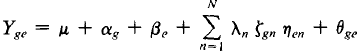
where Ysc, is the yield of genotype, g, in the environment, e; µis the grand mean; α_gis the genotype mean deviation; βisthe environment mean deviation;θ_geis residuals.λnis the eigen value of the PCA axis, n; (ζ_gnand η_enare the genotype and environmentPCA scores for the PCA axis, n; N is the number of PCA axes retained in the model; K is the Tukey concurrence constant ;γeis the environment slope on the genotype means; δgis the genotype slope on the environment means.

The least-squares fit the AMMI model for balanced data (equal replication) is obtained in two steps: (i) The main effects in the additive part of the model (grand mean, genotype means, and environment means) are analyzed by the ordinary ANOVA. This leaves a non-additive residual (namely the interaction). (ii) The interaction in the multiplicative part of the model is then analyzed by PCA. If all PCA axes were retained, the resulting full model would have as many degrees of freedom as the data and would consequently fit the data perfectly. The usual intent is, however, to summarize much of the interaction in just a few PCA axes (with N = 1 to 3), resulting in a reduced AMMI model that leaves a residual. Because they allow the use of F-tests to determine the significance of the PCA MS, degrees of freedom are calculated by the simple method of Gollob (1968): d f = G + E - 1 - 2n

4.2. AMMI interpretation:

After select the AMMI model, a study of adapt­ability and phenotypic stability of the biplot graphic would be designed. The bi­plot term refers to a type of graphic that contains two categories of points or markers(17).It was com­binations of the orthogonal axis of the interaction principal component analysis (IPCA). The biplot graphic in­terpretation could be based on the variation causes by the main additive effects of genotype and environment, and the multiplicative effect of the G × E interaction(3). The abscissa represents the main effects (overall aver­age of the variables of the genotypes evaluated) and the ordinate is the first interaction axis (IPCA1). In this case, the lower the IPCA1 value (absolute values), the lower its contribution to the G × E interaction; therefore, the more stable the genotype. The ideal genotype is one with high productivity and IPCA1 values close to zero. An undesirable genotype has low stability associ­ated with low productivity (Kempton, 1984; Gauch and Zobel, 1996; Ferreira et al., 2006). Finally, the predic­tive averages were estimated according to the selected model.

The significant effect of the G × E interaction revealed that the genotypes have been variable performance in the tested environments, i.e., a change in the av­erage rank of the genotypes verified among the environments, justifying the conduction of a more refined analysis so that to increase the efficiency of the selection and indication of cultivars. In this sense, AMMI analysis represents a potential tool that can be used to deepen the understanding of factors involved in the manifestation of the G × E interaction. Through this, it was estimated that the effect of the G × E interaction through multivariate analysis (principal components analysis, PCA and singular-value decom­position, SVD) could describe the pattern adjacent to the data from an interaction matrix (G × E), making the decomposition of the sum of squares of the G × E interaction (SSG×E) in axis or interaction principal components analysis (IPCA).

AMMI can be analysis by the different statistical tool of software’s, i.e. SAS, GenStat, R packages,etc.  The most flexible and easily available software to practices and early technology is R free software and its packages. Agricole package is good packages to analysis AMMI model.

5. Advantages and Disadvantages of AMMI:

5.1. Advantages of AMMI:

Several merits of AMMI were described through different stakeholders. Major several advantages are shortly described by Zobel et al. (1988); Guach and Zobel, (1996) listed as follows:

1. Methods for analyzing and G XE I to identify patterns of interaction
2. Used in extension of ordination with biplot and data validation.
3. Combines conventional ANOVA with Principal component analysis
4. May provides a more reliable estimate of genotype performance than mean across sites
5. Bi plot helps to visualize relationship among genotypes and environments; show both main and interaction effects.
6. Enables you to identify targets breeding environments to choose representative testing sites in those environments
7. Enables you to select varieties with good adaptation to target breeding environments
8. Can be used to identify key agro-climatic factors, disease, and insect pests, and physiological traits that determine adaptation to environments.
9. Based on a two-way matrix of genotypes x environments, combine ANOVA and PCA into single analysis with both additive and multiplicative statistical model.
10. Partition treatment SS into a model and residual which traditional approaches for controlling error, partition the error SS into pure error and blocks.
11. Possible to be done both errors of pure and blocks
12. Gains in precision due to modeling using AMMI are often several times as large as those due to blocking AMMI Disadvantages:
13. It is difficult to describe the GEI effects if number of components retained in the model is large (m ≥ 3).
14. Environmental response pattern cannot be estimated directly from AMMI model.
15. Estimating the next generation of environmental effect is difficult due to climate change, that means tell only the result of past effects.

6. Application of AMMI:

AMMI analysis is applicable when data are:

1. Quantitative rather than categorical
2. Significance main and interaction effects from ANOVA

           AMMI is divided into three major parts.

1. AMMI 0 = considers additive mean effects (genotypes and environmental means) to explain the data matrix, ranks genotypes identically at each environment, ignoring GE.
2. AMMI 1 = Considers main effects + the first two PC (PC 1) to interpret the residual matrix.
3. AMMI 2 = considers the main effects and the first two PC (PC 1 and PC2) for non-additive effects.

Practical Example of AMMI and Interpretation:

Twenty-two genotypes of Sorghum were planted at fourteen different environments to examined adaptation abilities. The harvested yield was analyzed by AMMI model. The ANOVA table with result was showed as followed in Table 2.  There is significance different between genotypes, environments and their interaction. Similarly, there is significant different between PC.

                                                                       Table 2: AMMI table

The biplot represented that, environments are distributed from lower yielding in quadrants I (top left) and IV (bottom left) to the higher yielding in quadrants II (top right) and III (bottom right) (Figure 1 and 2).

Accordingly, E12, E9, E1 and E14 were higher yielding environments for G5 and G.  Several genotypes, G21, G14, G12, G13 and G17 were specific higher yield to environments of E1 and E14. Lower yielding environments were E5, E10, and E11 with genotypes of G8, G1, G9, and G19 provided lower yield.  Furthermore, genotypes which located at the center of bi plots were more stable and adapted to wide environments.

Primary PC analysis included 28.9 % and second PC explained 16.8%.  Higher grain yield recorded per PCI were E12, E1 and lower yield obtained at E5 and E10.

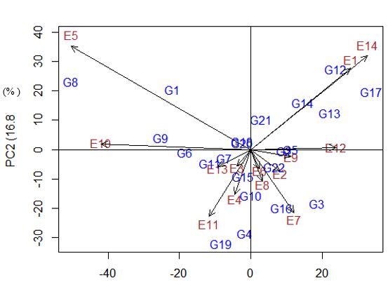
 Figure 1: Biplot explanation of yield and Environments with PCA.

Figure 2: Grain yield Vs only in PCA (%)1.

7. Conclusion:

To summarize, Additive main multiplicative model (AMMI) is a sophisticated method of genotype environmental interaction (GXEI) analysis in plant breeding experiments. The AMMI model is the combination of three different level of analysis which included analysis of variances (ANOVA), principle of component analysis (PCA) and visualized on the graph(3, 4).

It is frequently preferable at a condition of GXE interaction would be significance difference exist.  It is very useful to identify the participation of genotypes and environmental effects in multiplicative effects which fail to detect significant interaction with ANOVA.  Therefore, provided exact result affects of analysis which analysis of variance (ANOVA) and Linear Regression fails to detect a significant interaction component, principal component analysis (PCA) fails to identify and separate the significant genotype and environment main effects (Zobel et al., 1988).