Introduction:

COVID-19, a global pandemic, is an emerging disease that spreads from human to human and is responsible for infecting millions and killing thousands of people since the first reported fatal cases in late 2019. COVID-19 belongs to the family of zoonotic coronaviruses such as the Severe Acute Respiratory Syndrome coronavirus (SARS-Cov) and the Middle East Respiratory Syndrome (MERS-Cov) that have their origin in bats, mice, and domestic animals. The virus first emerged in Wuhan, the capital city of China’s Hubei province, in late December 2019. In just a few months, the virus spread rapidly across the world, reaching a total of approximately 4.7 million confirmed cases and 315,496 deaths as of 18 May 2020.[1] The first case of COVID-19 in India was reported in Kerala on the 30^th  of January 2020, with origins in China.[2] By 17 May 2020, India had registered a total of 95,698 confirmed cases and 30,24 deaths.[3]

As of today, the disease has spread all over the world. The number of confirmed COVID-19 cases vary due to the differences in the testing and disease surveillance capacities across the countries and regions. Since there is no valid treatment method and prevention for this virus yet, effective planning and proper implementation of the health infrastructure and services is the only way to control the spread of the virus. For this reason, accurate forecasting of future total confirmed cases plays a vital role in managing the health system and allows the decision-makers to develop a strategic plan and interventions to avoid a possible epidemic. Also, such estimates help in guiding the intensity and types of interventions needed to lessen the outbreak [.4,5] To estimate the number of additional manpower and resources needed to control the outbreak, a mathematical and statistical modeling tool is required that can be used for making short- and long-term disease forecasting.          

In the last few years, studies have used different statistical methods such as multivariate linear regression, [6] simulation-optimization approach, [7] generalized growth model and generalized logistic model, [8] holt method, [9] and grey model [10] to forecast epidemic cases. These statistical models, however, are inadequate for analyzing the influence of randomness on the epidemic outbreak. Random factors play an important role in the spread of a disease as Nakamura and Martinez have described in their study.[11]

Autoregressive integrated moving average (ARIMA) models are the most commonly used prediction models and are considered to be the best [12] for predicting epidemic diseases, such as malaria, [13] tuberculosis,[14] measles,[15] and influenza.[16] An ARIMA model is commonly used for predicting the time series data of infectious diseases, especially for series that have a cyclical or repeating pattern. Mostly, it deals with non-stationary time series in order to capture the linear trend of an epidemic or a disease, and it mainly predicts a future time series value by considering the previous time series values and the lagged forecast error.

In recent studies, different models have been used to predict the prevalence, incidence, and mortality rate of COVID-19. Perone (2020) used an ARIMA model and predicted that Italy would reach the inflection point in terms of cumulative cases during the months of April and May.[17] Zhao et al. (2020) applied the Metropolis-Hastings algorithm and predicted the effects of three epidemic intervention scenarios, that is, suppression, mitigation, and mildness in controlling the spread of COVID-19 in African countries. [18] Wang et al. (2020) used the SEIR model and virus reproduction rate R to predict the number of infectious cases in Wuhan, China.[4]

With the rising number of COVID-19 cases every day, there is a lot of stress on the administration and the health care system in India for accommodating patients with symptoms of COVID-19. Hence, the prediction of the estimated new cases in the coming days will help the health administration make adequate arrangements with ample time.       

This paper aims to forecast the prevalence of COVID-19 cases in Maharashtra, Delhi, and Kerala. The COVID-19 data corresponds to the period between 16 March 2020 and 27 June 2020. The best fit ARIMA model was used to estimate the prevalence of COVID-19 cases for a period of 30 days. In addition to highlighting the characteristics of the epidemic and the behavior of its spread, this study also provides the health authorities crucial information about the intensity of the epidemic at peak times using ARIMA model. These models can help predict the health infrastructure and materials the patients will need in the future.   

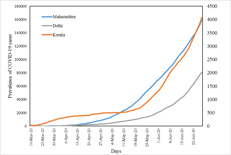
Figure: Represent the Prevalence of COVID-19 cases in Maharashtra, Delhi, and Kerala

Methods:

Data Source:

For the validation and analysis of the proposed study, the prevalence of COVID-19 cases was taken from the website www.covid19india.org and Microsoft Excel was used to build a time-series database. The minimum sample size required for time series forecasting is 30 observations. [19] Hence in this study, 104 time-series observations between 16 March 2020 and 27 June 2020 were used to predict the prevalence of COVID-19 cases over the next 30 days with a 95% confidence interval limit. All analyses were performed using Statgraphics Centurion XVII.II software, with p-value<0.05 as the statistical level of significance.

Statistical Analysis:

ARIMA Model:

A time series is a sequence of observations, each one being recorded at a specific time; it may be measured continuously or discretely.[19] The main aim of a time series is to study past observations and develop an appropriate model to forecast future values. The ARIMA model, first introduced by Box and Jenkins in the 1970s, is the most used time series model if the data show no seasonality pattern. The ARIMA model – generally represented as ARIMA(p,d,q) – is an extension of autoregressive AR(p), moving average MA(q), and ARMA(p,q) models. [16] The letters p, d, and q correspond to order of autoregression, degree of difference, and order of moving average respectively. [19] In an AR(p) model, the current time series value Yt is expressed as a linear combination of p past observations Yt-1  Yt-2……Yt-p and a random error εt,  together with a constant term. Similarly, in an MA(q) model, the current time series value Yt uses past q error terms εt-1 εt-2……εt as the explanatory variables. The general formula of AR(p) and MA(q) models can be expressed as in Eq (1) and (2) respectively.

Yt=C + ∅1Yt-1+ ∅2Yt-2 +……+ ∅pYt-p+ εt                                      (1)

Yt=μ + θ1εt-1+ θ2εt-2 +……+ θqεt-q+ εt                                        (2)

Here ∅i (i=1, 2...p) and θj (j=1, 2...q) are the autoregressive and moving average parameters respectively. Yt is the observed value at time t and εt the random error (or random shock) at time t. C is the constant term, and μ is the mean of the series. The random shock is assumed to be a white noise process, that is, a sequence of independent and identically distributed (i.i.d) random variables with mean zero and a constant variance σ2.[19]

The ARMA(p,q) model is a combination of AR(p) and MA(q) models in which the current time series value Yt is defined linearly in terms of its past p observations as well as the current and past q random shock, together with a constant term. The general formula of an ARMA(p,q) model can be expressed as in Eq (3).

Yt=C + ∅1Yt-1+ ∅2Yt-2 +……+ ∅pYt-p+ εt + θ1εt-1+ θ2εt-2 +……+ θqεt-q    (3)

Where C is a constant and εt-k (k=1, 2…q) are the values of the previous random shock. Time series analysis requires a stationary time series, that is, the series shows no fluctuation or periodicity with time.[12] In an ARIMA model, a non-stationary time series is made stationary by applying finite differencing to the time series. The differenced stationary time series can be modeled as an ARIMA model to perform an ARIMA forecasting. [16]  

Best fit model selection:

Once a model is generated, it is necessary to test the goodness of the model fit before forecasting future values. The accuracy of the model can be determined by comparing the actual values with the predicted values. In this study, we used three performance measures, namely Mean Absolute Error (MAE), Mean Absolute Percentage Error (MAPE), and Root Mean Square Error (RMSE), to test the forecasting accuracy of a particular model. Mathematically, these measures are expressed as in Eq (4), (5), and (6).

MAE= 1nt=1net                                 (4)

MAPE=1nt=1netyt x 100                      (5)

RMSE=1nt=1net2                              (6)

Where yt is the actual value at time t, and et is the difference between the actual and the predicted values? Also, n is the number of time points. Lower MAE, MAPE, and RMSE values indicate a model that best fits the data. [20]

 Steps involved in ARIMA modeling:

Four critical steps are involved in the ARIMA modeling, namely, identification, estimation, diagnostic checking, and forecasting. The first step is to check the seasonality and stationarity of the time series data by drawing a time series plot of the observed series with the corresponding time. A time series is considered as stationary if a shift in time doesn’t cause a change in the shape of the distribution, that is, the statistical properties such as mean, variance, and autocorrelation are constant over time. The stationarity of time-series data is important as it helps develop powerful techniques to forecast future values.[21] The second step is to construct the autocorrelation (ACF) and the partial autocorrelation (PACF) plots of the stationary time series to determine the order of the AR and MA processes. The ACF is the correlation between the observation at time t and the observation at a different time lag, while PACF is the amount of correlation between the current observation at time t and the observation at lag k that is not explained by the correlation at all lower-order lags (that is, lag<k).[21] The third step involves estimating the parameters of the best fit model, which is done using the performance measure criteria. The ACF plot of residuals, as well as the Box-Pierce test of white noise, were determined to evaluate the model goodness of fit. The fourth step involves forecasting future values using a good fit model.

Results:

Prevalence and incidence of COVID-19:

Table 1: Descriptive statistics of the Prevalence and Incidence of Covid-19 in Maharashtra, Delhi, Kerala, and India

The descriptive statistics of the prevalence and incidence of COVID-19 in Maharashtra, Delhi, and Kerala are given in Table 1. As seen in

Figure  1: Represent the Prevalence of COVID-19 cases in Maharashtra, Delhi, and Kerala
Figure 1 the prevalence curve of COVID-19 has been growing at a steep rate, with the states of Maharashtra and Delhi following a similar trend. With an average of 1530 new cases per day Maharashtra was one of the most hard-hit states of India. In the national capital Delhi, the first case of COVID-19 was reported on the 2^nd of March, and since then, the number of confirmed cases has climbed to about 80,188 cases. 

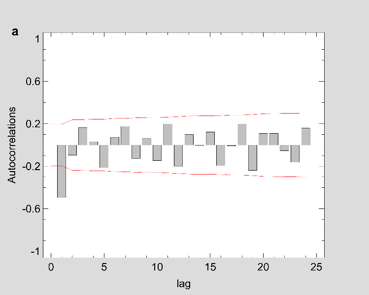
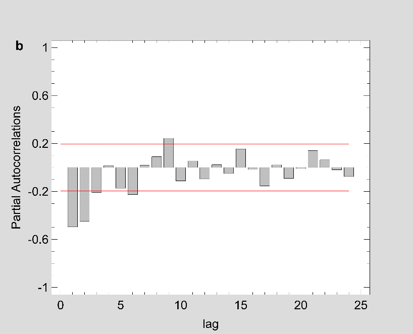
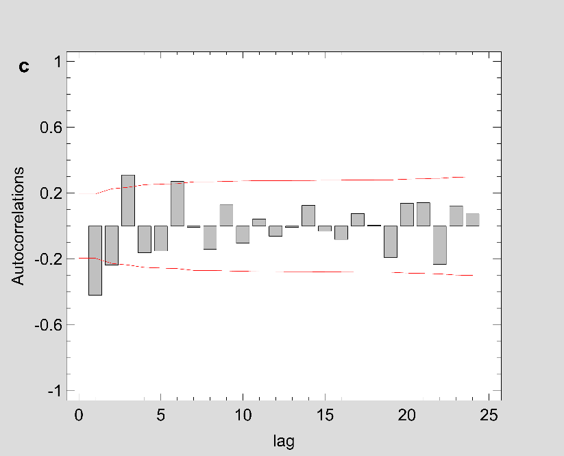
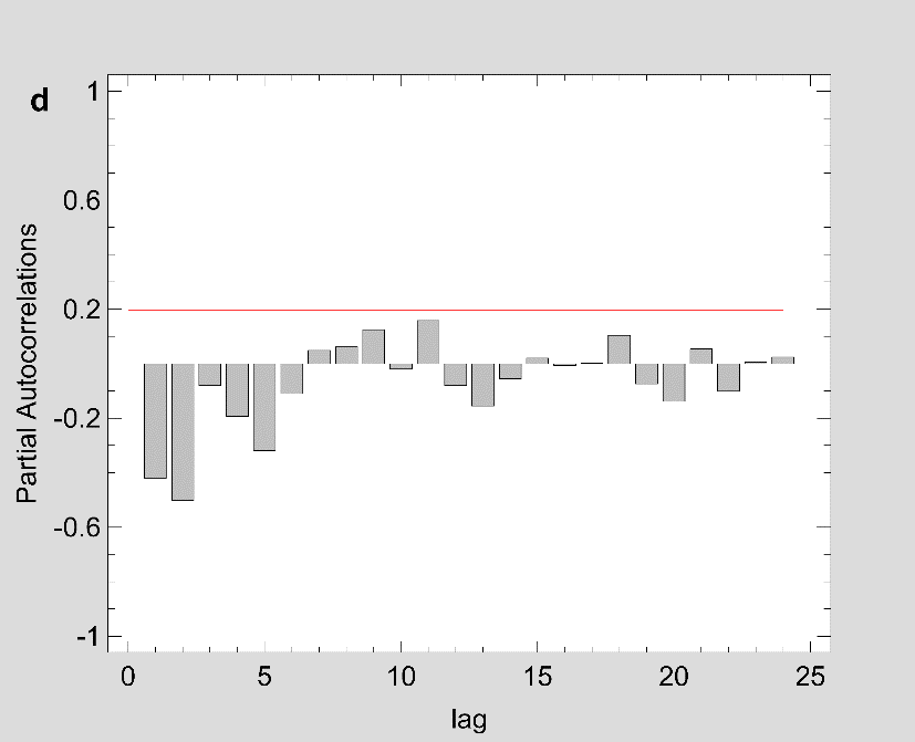
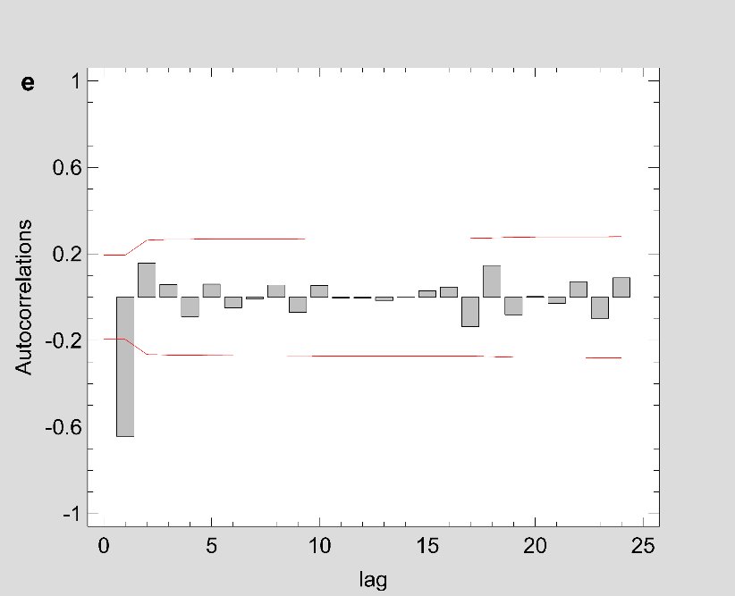
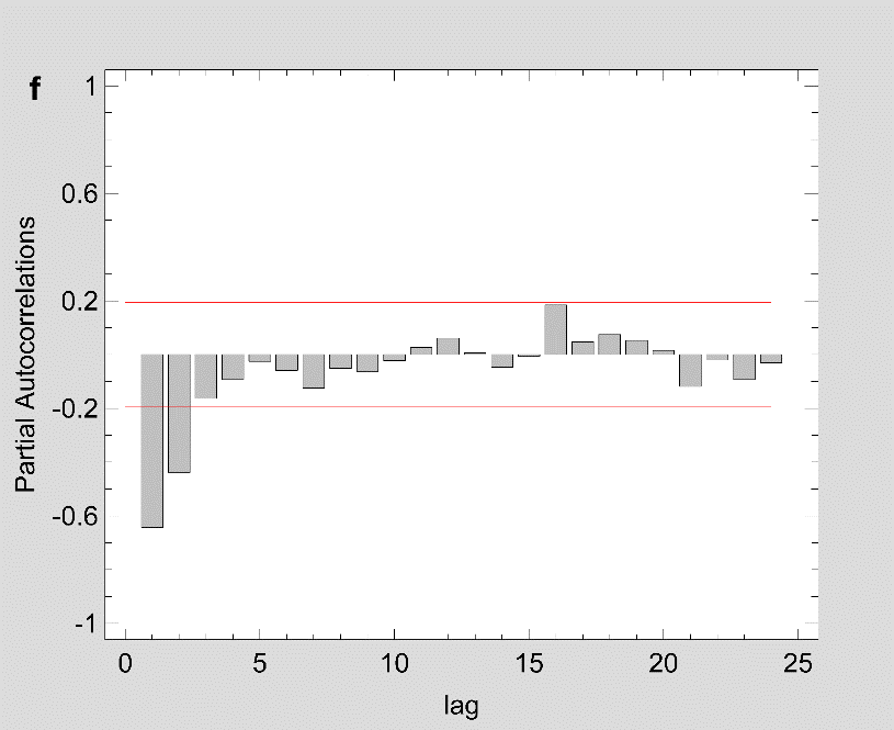
Figure  2: The estimated ACF and PACF plot to predict the trend of Covid-19 prevalence for (a-b) Maharashtra (c-d) Delhi and (e-f) Kerala.

Note: Figure 2 should be black and white print
Forecasting the prevalence of COVID-19 pandemic using the time series ARIMA model:

Table 2: Comparison of ARIMA models performance measures.

Table 3: Parameters of best fit ARIMA models.

Fig 1 show that the prevalence of COVID-19 in this study shows no seasonal pattern, which is also supported by the autocorrelation plot of the cumulative COVID-19 cases for Maharashtra, Delhi, Kerala (see Appendix). The two lines on the graph indicate the lower and upper limits of the 95% confidence interval. These lines help identify the presence of non-zero autocorrelation. The ACF plot confirms that the prevalence of COVID-19 is not stationary as the autocorrelation is seen to reduce slightly with increasing lag (see Appendix). The first- and second-order differencing were taken to stabilize the mean of COVID-19 prevalence for Maharashtra, Delhi, Kerala. After the third-order differencing, the series became stationary, and the parameters of the ARIMA model were determined according to the ACF and PACF plots as shown in Fig  2. All the analyses were performed on the transformed prevalence of COVID-19. The ARIMA model with the lowest MAPE and with most statistically significant parameters was selected as the best model for forecasting. ARIMA (1,3,1), ARIMA (2,3,2), and ARIMA (2,3,1) were selected as the best fit models for Maharashtra, Delhi, and Kerala. With the MAPE _Maharashtra= 3.4, MAPE _Delhi= 13.615, and MAPE _Kerala= 2.011, the models fitted the prevalence of COVID-19 very well (Fig  2 and Table 2). All the estimated parameters of the best fit models are presented in Table 3. The fitted and predicted total confirmed COVID-19 cases are presented in Table 4 and Fig  3. For the next 30 days, the total number of confirmed COVID-19 cases is estimated to be from 3,60,888 to 5,18,538 in Maharashtra, 1,63,017 to 2,52,929 in Delhi, 10,023 to 14,204 in Kerala.

Table 4: Prediction of the total confirmed Covid-19 cases for the next 30 days according to ARIMA models with 95% confidence interval

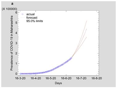
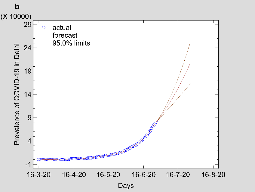
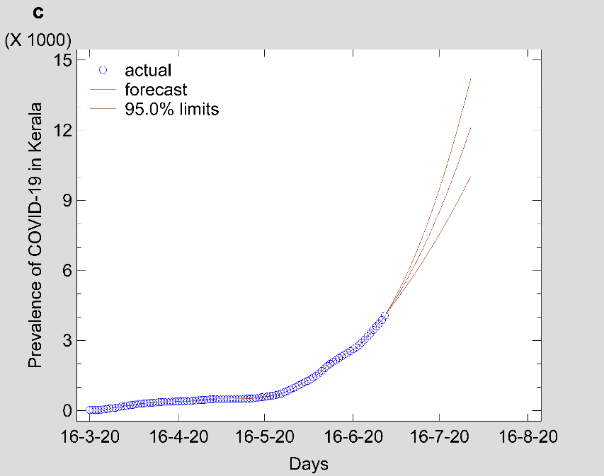
Figure  3: Time series forecasting plot estimated from ARIMA best-fit model for (a) Maharashtra (b) Delhi and (c) Kerala.

Note: Fig 3 should be black and white print

Discussion:

In an effort to slow down the spread of COVID-19, the Indian government took strong measures by announcing a countrywide lockdown on 24 March 2020 as the number of confirmed positive cases were increasing in the country. Estimating the prevalence and intensity of an epidemic is crucial for allocating medical and health resources, production of activities, and even the economic situation of the country. Hence developing a forecasting model that accurately predicts the future intensity of an epidemic can help the government administrators and decision-makers prepare the manpower and medical supplies required during an outbreak. In this study, the ongoing trend and the intensity of the COVID-19 pandemic were estimated using the ARIMA time series model. The ARIMA model is one of the best models and has been extensively employed to predict the incidence of contagious diseases. [22] To the best of our knowledge, this is the first study in India to apply the ARIMA model to estimate the prevalence of COVID-19 in India major states.

India has reported a lower COVID-19 death rate as compared to countries like China, United Kingdom, Italy, Spain, and the United States. [23] However, the total confirmed COVID-19 cases in most of the Indian states show no sign of a downward trend. At the time of writing this article, India had 5,38,529 positive confirmed cases [3] and was expected to overtake Russia total COVID-19 cases. Minhas (2020), in his study, points out that India is another potential epicenter of the global COVID-19 pandemic due to human overpopulation and unhygienic living conditions. ²⁴ Containing the spread of the virus among the economically disadvantaged people, who may not be able to self-isolate, is a challenge. In Maharashtra, the number of daily new cases since March 16 has grown exponentially and crossed the 1000-cases-per-day mark on May 6. Mumbai, the state capital of Maharashtra and also India’s financial capital, has been the worst hit city by COVID-19, having recorded 15,750 total cases accounting for 20 percent of all positive COVID-19 cases in India.²⁵ Kerala reported the first case of COVID-19 in India; however, over a period of one month, the daily new confirmed cases significantly reduced to zero for five consecutive days.³ Delhi, the national capital, reported 3947 COVID-19 cases in a single day on June 23, the highest jump so far. With the lockdown curbs being relaxed after May 17, the number of new cases may increase further.²⁶ This pattern will burden the health system to its maximum capacity. As a result, if adequate measures to contain the spread are not appropriately enforced, and social distancing is not maintained, the number of cases is not expected to plateau any time soon.

An epidemic is a numbers game and as far as numbers are concerned, India has a handful of them. With no valid medical treatment and preventive measures for this virus to date, forecasting the prevalence of the disease is a vital strategy to strengthen the surveillance and allocate health resources accordingly. The results of the study will help health authorities and health care management plan the necessary supply resources, which include medical staff, medical equipment, intensive care facilities, hospital beds, and other healthcare facilities. This will make the epidemic controllable and bring it within the domain of the available healthcare resources in India.  

Acknowledgments:

Conflict of interest statement: The authors declare that they have no conflicts of interest.

Role of funding source: The research did not receive any specific grant from funding agencies in the public, commercial, or not-for-profit sectors.

Ethical Approval: Non sought